Summary¹: The likelihood function implied by an estimate $b$ with standard deviation $\sigma$ is the probability density function (PDF) of a $\mathcal{N}(b,\sigma^2)$. Though this might sound intuitive, it’s actually a special case. If we don’t firmly grasp that it’s an exception, it can be confusing.

Suppose that a study has the point estimator $B$ for the parameter $\Theta$. The study results are an estimate $B=b$ (typically a regression coefficient), and an estimated standard deviation² $\hat{sd}(B)=s$.

In order to know how to combine this information with a prior over $\Theta$ in order to update our beliefs, we need to know what is the likelihood function implied by the study. The likelihood function is the probability of observing the study data $B=b$ given different values for $\Theta$. It is formed from the probability of the observation that $B=b$ conditional on $\Theta=\theta$, but viewed and used as a function of $\theta$ only³:

The event “$B=b$” is often shortened to just “$b$” when the meaning is clear from context, so that the function can be more briefly written $\mathcal{L}: \theta \mapsto P(b \mid \theta)$.

So, what is $\mathcal{L}$? In a typical regression context, $B$ is assumed to be approximately normally distributed around $\Theta$, due to the central limit theorem. More precisely, $\frac{B - \Theta}{sd(B)} \sim \mathcal{N}(0,1)$, and equivalently $B\sim \mathcal{N}(\Theta,sd(B)^2)$.

$sd(B)$ is seldom known, and is often replaced with its estimate $s$, allowing us to write $B\sim \mathcal{N}(\Theta,s^2)$, where only the parameter $\Theta$ is unknown⁴.

We can plug this into the definition of the likelihood function:

We could just leave it at that. $\mathcal{L}$ is the function⁵ above, and that’s all we need to compute the posterior. But a slightly different expression for $\mathcal{L}$ is possible. After factoring out the square,

we make use of the fact that $(b-\theta)^2 = (\theta-b)^2$ to rewrite $\mathcal{L}$ with the positions of $\theta$ and $b$ flipped:

We then notice that $\mathcal{L}$ is none other than

So, for all $b$ and for all $\theta$, $\mathcal{L}: \theta \mapsto \text{PDF}_{\mathcal{N}(\theta,s^2)}(b) = \text{PDF}_{\mathcal{N}(b,s^2)}(\theta)$.

The key thing to realise is that this is a special case due to the fact that the functional form of the normal PDF is invariant to substituting $b$ and $\theta$ for each other. For many other distributions of $B$, we cannot apply this procedure.

This special case is worth commenting upon because it has personally lead me astray in the past. I often encountered the case where $B$ is normally distributed, and I used the equality above without deriving it and understanding where it comes from. It just had a vaguely intuitive ring to it. I would occasionally slip into thinking it was a more general rule, which always resulted in painful confusion.

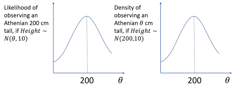
To understand the result, let us first illustrate it with a simple numerical example. Suppose we observe an Athenian man $b=200$ cm tall. For all $\theta$, the likelihood of this observation if Athenian men’s heights followed an $\mathcal{N}(\theta,10)$ is the same number as the density of observing an Athenian $\theta$ cm tall if Athenian men’s heights followed a $\mathcal{N}(200,10)$⁶.

Graphical representation of $\text{PDF}_{\mathcal{N}(\theta,10)}(200) = \text{PDF}_{\mathcal{N}(200,10)}(\theta)$

When encountering this equivalence, you might, like me, sort of nod along. But puzzlement would be a more appropriate reaction. To compute the likelihood of our 200 cm Athenian under different $\Theta$-values, we can substitute a totally different question: “assuming that $\Theta=200$, what is the probability of seeing Athenian men of different sizes?”.

The puzzle is, I think, best resolved by viewing it as a special case, an algebraic curiosity that only applies to some distributions. Don’t even try to build an intuition for it, because it does not generalise.

To help understand this better, let’s look at at a case where the procedure cannot be applied.

Suppose for example that $B$ is binomially distributed, representing the number of successes among $n$ independent trials with success probability $\Theta$. We’ll write $B \sim \text{Bin}(n, \theta)$.

$B$’s probability mass function is

Meanwhile, the likelihood function for the observation of $b$ successes is

To attempt to take the PMF $g$, set its parameter $\theta$ equal to $b$, and obtain the likelihood function would not just give incorrect values, it would be a domain error. Regardless of how we set its parameters, $g$ could never be equal to the likelihood function $\mathcal{M}$, because $g$ is defined on $\{0,1,...,n\}$, whereas $\mathcal{M}$ is defined on $[0,1]$.

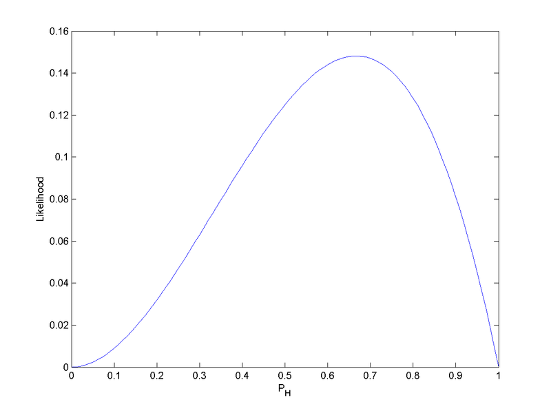
The likelihood function $\mathcal{Q}: P_H \mapsto P_H^2(1-P_H)$ for the binomial probability of a biased coin landing heads-up, given that we have observed $\{Heads, Heads, Tails\}$. It is defined on $[0,1]$. (The constant factor $3 \choose 2$ is omitted, a common practice with likelihood functions, because these constant factors have no meaning and make no difference to the posterior distribution.)

It’s hopefully now quite intuitive that the case where $B$ is normally distributed was a special case.⁷

Let’s recapitulate.

The likelihood function is the probability of $b\mid\theta$ viewed as a function of $\theta$ only. It is absolutely not a density of $\theta$.

In the special case where $B$ is normally distributed, we have the confusing ability of being able to express this function as if it were the density of $\theta$ under a distribution that depends on $b$.

I think it’s best to think of that ability as an algebraic coincidence, due to the functional form of the normal PDF. We should think of $\mathcal{L}$ in the case where $B$ is normally distributed as just another likelihood function.

Finally, I’d love to know if there is some way to view this special case as enlightening rather than just a confusing exception.

I believe that to say that a $\text{PDF}_{\theta,\Gamma}(b)=\text{PDF}_{b,\Gamma}(\theta)$ (where $\text{PDF}_{\psi,\Gamma}$ denotes the PDF of a distribution with one parameter $\psi$ that we wish to single out and a vector $\Gamma$ of other parameters), is equivalent to saying that the PDF is symmetric around its singled-out parameter. For example, a $\mathcal{N}(\mu,\sigma^2)$ is symmetric around its parameter $\mu$. But this hasn’t seemed insightful to me. Please write to me if you know an answer to this.