A mathematical model for Value of Information
Summary: I developed a piece of software to numerically estimate the expected payoff from receiving a signal, i.e. the expected value of information (EVOI), in a simplified model. In this post, I explain the model, and walk through an example where we want to know the EVOI of funding a clinical trial of an HIV drug that could improve upon antiretroviral therapy (ART). With a prior that implies a 23% chance that the new drug is truly more effective than ART, I find that we should be willing to pay over $800M for a clinical trial that would influence $5bn of funding.
Background
Researchers at Open Philanthropy and I were interested in the question of whether and how much Open Philanthropy should fund studies, such as clinical trials or field randomised controlled trials (RCTs), to generate information that would help direct philanthropic or government resources to their best use. We thought formal value of information (VOI) models might help inform that question. Outside of the special case where our prior is conjugate to our information, the VOI does not have an analytic expression. Instead I developed a piece of software for Open Philanthropy to numerically estimate the VOI (in a simplified model). Because the concept of VOI is quite general and my code is extensible, we hope that the tool can also be useful to others beyond Open Philanthropy. I also had a huge amount of fun on this project.
What is value of information? When we gain information about a decision-relevant quantity, that information may improve the decision we ultimately make. The value of the (expected) improvement in the decision is the (expected) value of information (EVOI).
Sometimes, the information we gain tells us that one action is certain to be better than another (for example, if I’m late for the airport, and I learn my flight has already departed, there is no longer any point in rushing). But often, the information is imperfect, and can only pull our decision in the direction of optimality, in expectation.
Such imperfect information can be modelled as observing a random variable (or signal) B that is informative about the true value of an unobservable quantity T1 but contains some noise. The expected value of information is the expected benefit from observing this random variable.
The realised value of information in a state of the world T, B is:
VOI(T,B) = U(decision(B), T) - U(decision_0, T)
where U is the payoff function, decision is the decision function when we have access to the signal, and decision_0 is the decision we make in the absence of the signal.
The EVOI is V=E[VOI(T,B)], where the expectation is taken with respect to the joint distribution of T and B.
I have written a Python package and accompanying website that sets up a simplified model and calculates V in that model. It uses Monte Carlo methods (i.e. random sampling from the distribution of T and B).
The model
I’ll just tell you the bare minimum about the model setup; everything is explained in detail in the documentation of the package.
We model the decision problem as a binary choice is between:
- the funding bar : an option with an expected payoff of
barabout which we cannot gain additional information (for example, the effectiveness of a well-established method such as antiretroviral therapy for HIV). - the object of study: an uncertain option whose payoff is
T, about which we can gain additional information through the signalB(for example, a speculative new HIV treatment that we are considering funding a clinical trial of).
B is normally distributed around the unobservable T. The central limit theorem makes this assumption reasonable for large samples or if measuring a quantity that is normally distributed to begin with.
We model a rational decision-maker, i.e. upon receiving a signal of B=b they update their prior P(T) to P(T|B=b). They risk-neutrally maximise expected U, which means they choose the object of study if and only if the posterior expected value E[T|B=b]>bar (in the absence of the signal, they choose the object of study if and only if the prior expected value E[T]>bar).
There’s obviously nothing inherent in this model that makes it specific to philanthropy. It could be applied to any topic. There are a few other restrictions in my model (see documentation) but the code should be relatively easy to extend to new sets of assumptions. Pull requests are welcome!
Example: HIV treatment
Let’s walk through the example of HIV treatments in a lot more detail. I am mostly interested in explaining the mechanics of the model and how you might interpret its conclusions, so this example isn’t meant to be highly realistic, but I hope it does not feel completely toy. I will try to use numbers that are not outrageously (»10x) distant from the truth.
Suppose we are a philanthropic funder of HIV/AIDS interventions. Antiretroviral therapy (ART) is a well-established intervention to control an HIV infection and prevent progression to AIDS. We are considering funding a clinical trial of a speculative new drug (the object of study) that could be scaled up if it were more cost-effective than antiretroviral therapy (the bar).
Before thinking about cost-effectiveness, we can first think about simple effectiveness in increasing life expectancy. Let’s suppose that ART increases life expectancy by 10 years compared to no treatment2, so the bar is 10 years3.
Suppose our prior over the effectiveness T of the speculative drug is a lognormal distribution with mu=1.7 and sigma=0.8. This implies the prior expected value is 7.5 and we assign a 23% chance that the drug beats antiretrovirals. Because the expected value of 7.5 is less than the bar of 10, we would not fund the speculative drug in the absence of additional information.

We’re considering a study with 49 participants4, which assuming a standard deviation of life expectancy of 21 years5, gives sd(B)=21/sqrt(49)=3. That’s all we need to run our simulation:
prior_mu, prior_sigma = 1.5, 1
prior = lognormal(prior_mu, prior_sigma)
params = SimulationParameters(prior=prior, sd_B=3, bar=10)
simulation_run = SimulationExecutor(params).execute()
The results show that this study gives an EVOI of about 2 years. This means that by running the study, in expectation we can extend the lifespans of a patient by an additional 2 years on top of the 10 years available with ART.
Mean VOI 2.0338
We can also see that our subjective posterior expected value for the speculative intervention can be expected to beat ART 20% of the time.
Fraction of iterations where E[T|b_i] > bar 0.1898
Moreover, we can plot the probability that the subjective posterior expected value is greater than bar as a function of T, in other words the probability that we choose the speculative drug as a function of the unobservable T.6

Or, we can look at the decision-maker’s subjective posterior expected value as a function of the signal:

Cost-benefit analysis
We can now turn to the cost-benefit analysis. The model of costs and benefits that I wrote is independent of the VOI calculations.
The model is well-suited when choosing between different options that can absorb flexible amounts of capital (e.g. philanthropy, investing, or ad spend).
The cost-benefit analysis assumes:
- “Choosing” the bar or the object of study means spending 100% of one’s remaining capital implementing that option. (This is only optimal if there are no diminishing returns).
Tandbarshould now be expressed in terms of cost-effectiveness (i.e. value realised per unit of capital).- The decision-maker can choose to spend
signal_costto acquire the signal. All other capital is spent implementing the option with the highest expected value.
We need to shift our units from effectiveness (years of life expectancy added) to cost-effectiveness (years added per $M spent). We can suppose that
- ART and the speculative drug both cost $0.1M ($100,000) over a lifetime
The bar is now 100 years per $1M. The prior is now a LogNormal(mu=1.5+log(10), sigma=1)and sd(B)=307.
With the new parameters, we get an EVOI of 20 years per million dollars:
Mean VOI 20.6088
As expected, this is the previous EVOI divided by 0.1M$.
We can now enter the cost-benefit parameters. Since this can get a little confusing, the program makes us explicitly enter all the units, and displays the units back to us:
cb_params = CostBenefitParameters(
	value_units="years added",
	money_units="M$",
	capital=???,
	signal_cost=11,
)
Let’s say that the study costs $ 11M 8. We also need to know how much capital is available to potentially be infuenced by the information. Setting the capital parameter is the trickiest part of applying this model to philanthropy. The key point is that in philanthropy other actors share our goals and the results of the study will be released publicly. We need to worry not just about our own capital (which we are sure would shift based on the results of the study), but about the total pool of capital that may be influenced in the same way. In practise, it’s difficult to know how other funders will react to information. We’ll have uncertainty over that, so we’re really estimating influencable capital as a sum over different pots of capital, weighted by the probability these pots will shift what they fund according to rational updating from a prior of P(T).9 Let us nevertheness say that $ 5,000M ($ 5 billion) would be influenced by the study.
We can now run it:
CostBenefitsExecutor(inputs=cb_params, simulation_run=simulation_run).execute()
Best option without signal (years added per M$ spent)            100
Capital (M$)                                                   5 000
Expected value without signal (years added)                  500 000
Expected benefit from signal (years added per M$ spent)           20
Capital left after signal (M$)                                 4 989
Expected value with signal (years added)                     600 331
Expected net benefit from signal (years added)               100 331
The benefits greatly exceed the costs. We would break even if we spent $853M on the study:
Willingness to pay for signal (M$) 863
For a capital of $1bn, this willingness to pay is still $167M:
Willingness to pay for signal (M$) 167
Note that this is not driven by the fact that ART is a miraculous technology; none of the value here comes from giving ART to patients who would otherwise not have had it. This is because we assumed that the costs of the two interventions are the same, so the $5bn gives treatment to 50,000 patients regardless of which intervention is chosen.
How VOI is distributed
Marginal distribution of VOI
The package also tells us the distribution of VOI
Quantile 0.01 VOI                            -2.2
Quantile 0.05 VOI                             0.0
Quantile 0.1 VOI                              0.0
Quantile 0.25 VOI                             0.0
Quantile 0.5 VOI                              0.0
Quantile 0.75 VOI                             0.0
Quantile 0.9 VOI                              5.1
Quantile 0.95 VOI                            10.5
Quantile 0.99 VOI                            25.2
We can see that the VOI is sometimes negative (2.9% of the time, in fact). We can get an unlucky draw, where the study results B=b are so far from the truth T=t that the study causes us to make the wrong decision when we otherwise would not have. In this case, this would mean choosing the speculative drug when its true effect is less than 10 years.
(You may have the intuition that VOI cannot be negative: after all, if our information is worse than no information, we can just ignore it! This is consistent with what I am saying. By VOI I mean VOI(b,t), the realised VOI in a particular state of the world b,t, you can get unlucky with that state and get negative VOI. It is only the expected VOI V that cannot be negative.)
We can confirm this understanding by inspecting some of the draws where the VOI was negative (d_1 is shorthand for the decision of choosing the bar and d_2 for choosing the object of study).
  T     B no_signal  U_no_signal w_signal  U_w_signal E[T|B]>bar    VOI   B-T
7.5  11.9       d_1           10      d_2         7.5       True   -2.5   4.3
9.5  11.9       d_1           10      d_2         9.5       True   -0.5   2.5
7.9  12.7       d_1           10      d_2         7.9       True   -2.1   4.8
8.1  12.2       d_1           10      d_2         8.1       True   -1.9   4.2
7.8  11.9       d_1           10      d_2         7.8       True   -2.2   4.1
8.4  13.3       d_1           10      d_2         8.4       True   -1.6   4.9
3.4  12.5       d_1           10      d_2         3.4       True   -6.6   9.2
5.5  13.1       d_1           10      d_2         5.5       True   -4.5   7.6
9.4  13.7       d_1           10      d_2         9.4       True   -0.6   4.3
7.2  12.0       d_1           10      d_2         7.2       True   -2.8   4.8
In this tiny sample, can see that this happened when the distance B-T was between 2.5 and 9. These distances are positive, and large relative to sd(B)=3. A 1-sigma event of B-T≥3 happens 16% of the time, and a 2-sigma event of B-T≥6 happens 2% of the time, yet these are 90% and 20% of our sample, respectively.
We can view a histogram of VOIs. Because the VOI is nonzero only 20% of the time, the y-axis has been truncated for readability.

VOI in relation to T and B
We can also see the contribution to the VOI of different T-values, i.e. a graph of VOI(t)*P(T=t) (where VOI(t) means E[VOI(t,B) | T=t] ). This shows us that T-values of 20 years or higher (the 95th percentile of our prior) account for a large chunk of the VOI.

You may also have noticed that there is still a significant VOI contribution from very extreme values of >60. A 60-year improvement in life expectancy is clearly implausible. This tells us that our lognormal prior has implausibly fat tails (recall that the 77th percentile, only 10 years, seemed reasonable to us). This package supports priors of any functional form, so we can change the prior to something more reasonable, but I will leave that aside until the next section (see below).
It could also be useful to further develop intuition by plotting VOI against T and B. We see that the VOI is either 0, or it falls on a line whose coordinates are described by T-bar (in this case T-10).

The graph above deliberately uses different dark-light scales for zero and nonzero values, so that we can see the distribution within nonzero-VOI values, otherwise completely obscured by the distribution of zero-VOI values. Alternatively, we can use double histogram at the top of the graph (showing the marginal distribution of T), to compare the relative weight of zero and nonzero values for different T. I’ve reproduced that histogram below in a larger size. (This histogram is related to the earlier plot of the probability of each decision as a function of T: the VOI is nonzero if and only if we choose the object of study10. In terms of the plot below, the earlier plot showed the height of the orange bar divided by the height of the blue bar.)

We can also plot VOI against B, or against the noise component B-T of the study result. The VOI is negatively correlated with the noise. With a larger positive noise, we are more likely to be misled by the study into choosing the speculative drug, resulting in negative VOI. A large negative noise also makes us update our beliefs in the wrong direction, but we then just choose ART, so our final decision is no worse than it would have been. (Had the expected value of the prior been greater than the bar, we would see a positive correlation here).

{:width=”49%”} 
We can also plot the results in 3 dimensions, either as contour plots or surface plots.

Varying the prior
We noted earlier that our lognormal prior has implausibly fat tails. With our log normal, 1.6% of the time, T is greater than 30 years, an implausible increase in life expectancy. And these extreme values drive a lot of the VOI. The mean VOI when excluding T>30 is only about 1 year instead of 1.5 years.
The good news is this package supports arbitrary priors. We can choose a metalogistic prior with:
- a 5th percentile of 0 years (meaning a 5% chance of doing harm)
- a 77th percentile of 10 years (corresponding to the same 23% chance of beating ART as before)
- a 97.5th percentile of 20 years
- an upper bound of 30 years

prior = MetaLogistic(ubound=30, cdf_ps=[0.1, 0.77, 0.975], cdf_xs=[0, 10, 20])

params = SimulationParameters(prior=prior, sd_B=3, bar=10)

simulation_run = SimulationExecutor(params).execute()
We now get an EVOI of about 1 year:
Mean VOI                                      0.954

Fraction of iterations where E[T|b_i] > bar   0.021

Quantile 0.01 VOI                            -2.420
Quantile 0.05 VOI                             0.000
Quantile 0.1 VOI                              0.000
Quantile 0.25 VOI                             0.000
Quantile 0.5 VOI                              0.000
Quantile 0.75 VOI                             0.000
Quantile 0.9 VOI                              4.642
Quantile 0.95 VOI                             7.616
Quantile 0.99 VOI                            12.070
The cost-benefit analysis yields a willingness to pay of $435M:
prior = MetaLogistic(ubound=300, cdf_ps=[0.1, 0.77, 0.975], cdf_xs=[0, 100, 200])
params = SimulationParameters(prior=prior, sd_B=30, bar=100)
Best option without signal (years added per M$ spent)          100
Capital (M$)                                                  5000
Expected value without signal (years added)                 500000
Expected benefit from signal (years added per M$ spent)       9.54
Capital left after signal (M$)                                4989
Expected value with signal (years added)                    546542
Expected net benefit from signal (years added)               46542
Willingness to pay for signal (M$)                             435
Here are all the same plots, for the metalogistic prior:


How EVOI depends on the model parameters
I’ll demonstrate this by keeping the priors and varying sd(B) and bar. We could also vary the prior of course.
We know intuitively that the expected payoff of the signal (EVOI) is decreasing in sd(B).
It may also be intuitive that EVOI as a function of bar should follow an inverted U shape. With an extremely high or extremely low bar, the information has no chance of changing our behaviour; the information is most useful when the bar is in the middle region, over which we have high prior uncertainty. In fact, I believe the bar and prior combination that maximises EVOI is when the bar is equal to the prior expectation.
Metalog prior

Lognormal prior

-
It would be conventional to use here, but I choose
Tbecause it’s easy to distinguishTfromtin all situations, while unambiguously distinguishing from requires LaTeX. GitHub’s README files don’t support LaTeX and nor does Python out of the box. ↩ -
GiveWell writes: “Our best guess is that ART increases life expectancy by about 18 years compared to no treatment, but we have not yet investigated this question in detail. Our current estimate comes from comparing a cohort study of the life expectancy of patients receiving ART in Uganda, with a cohort study of the life expectancy of untreated patients in Uganda before ART was rolled out”. ↩
-
One way in which this model is clearly unrealistic is that, for a study of life expectancy, we need very long-term follow-up (such as a 20-year follow up). But by the time the study completes, the world will have changed a huge amount, which would change our funding bar. You’ll have to suspend disbelief and bear with me on that! ↩
-
I originally thought the mean life expectancy among 49 people with HIV may not be that likely to be normally distributed, but it actually does not look too bad, at least for the general population in a rich country. Based on US Social Security life tables, and applying the bootstrap method, I get this distribution, which has a mean of 78 and a standard deviation of 3.7 (data, code):
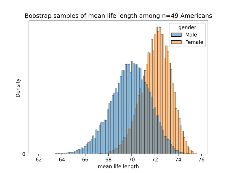
I did not want to select a larger sample size (where normality would definitely be reasonable) because with such a low-information prior, a much more precise signal than
sd(B)=3would mean the posterior expected valueE[T|B=b]is almost equal to the observed signalb, i.e. we almost entirely ignore our prior when making the decision. This would be terrible for expository purposes, you might inspect the data and get confused, thinking that no belief update is happening. ↩ -
The standard deviation in adult life span is about 15 years in the USA. I’m trying to use round numbers here. ↩
-
Mathematically,
P( E[T|B=b] > bar | T=t); the nested operators can make it seem like we’re taking the expectation of a constant, but we are not. In the inner expectation operator,bis taken as a constant andTas a random variable. We can re-write the eventE[T|B=b] > barasb>βfor some constant thresholdβ, which makes it explicit that that in the outer probability operatorP(b>β | T=t),bis taken as a random variable dependent onT. ↩ -
Previously,
T’s logarithm had a mean of 1.5 and a standard deviation of 1. How, we are consideringT'=T/0.1=10*T. We can take logs and getlog(T')=log(10) + log(T), after taking expectations we getmu=E[log(T')]=log(10) + E[log(T)]. For the standard deviationvar(log(T')) = var(log(10) + log(T))=var(log(T)), so thesigmaparameter is unchanged.Binstead is normally distributed, sovar(B') = var(10 * B) = 10^2 * var(B)and thussd(B')=10*sd(B). ↩ -
To caricature, we can say that we need to pay for 50 lifetime supplies of the drug ($5M) plus the fully loaded cost of a team of 3 people for 20 years ($6M). ↩
-
If we have a lot of knowledge about other funders, we could model another funder as acting according to its own prior
Q(T), but calculate the VOI by our lights, i.e. by the lights of someone who believesP(T). This meansTare drawn fromP(T)but the decision-maker we model acts according toQ(T). This isn’t currently supported out of the box by the package, but it could be added easily, or you could cobble it together based on combining multiple simulations. ↩ -
…given that the prior expected value
E[T]<bar. Mutatis mutandis forE[T]>bar. ↩
