Diagrams of linear regression

I made a big diagram describing some assumptions (MLR1-6) that are used in linear regression. In my diagram, there are categories (in rectangles with dotted lines) of mathematical facts that follow from different subsets of MLR1-6. References in brackets are to Hayashi (2000).

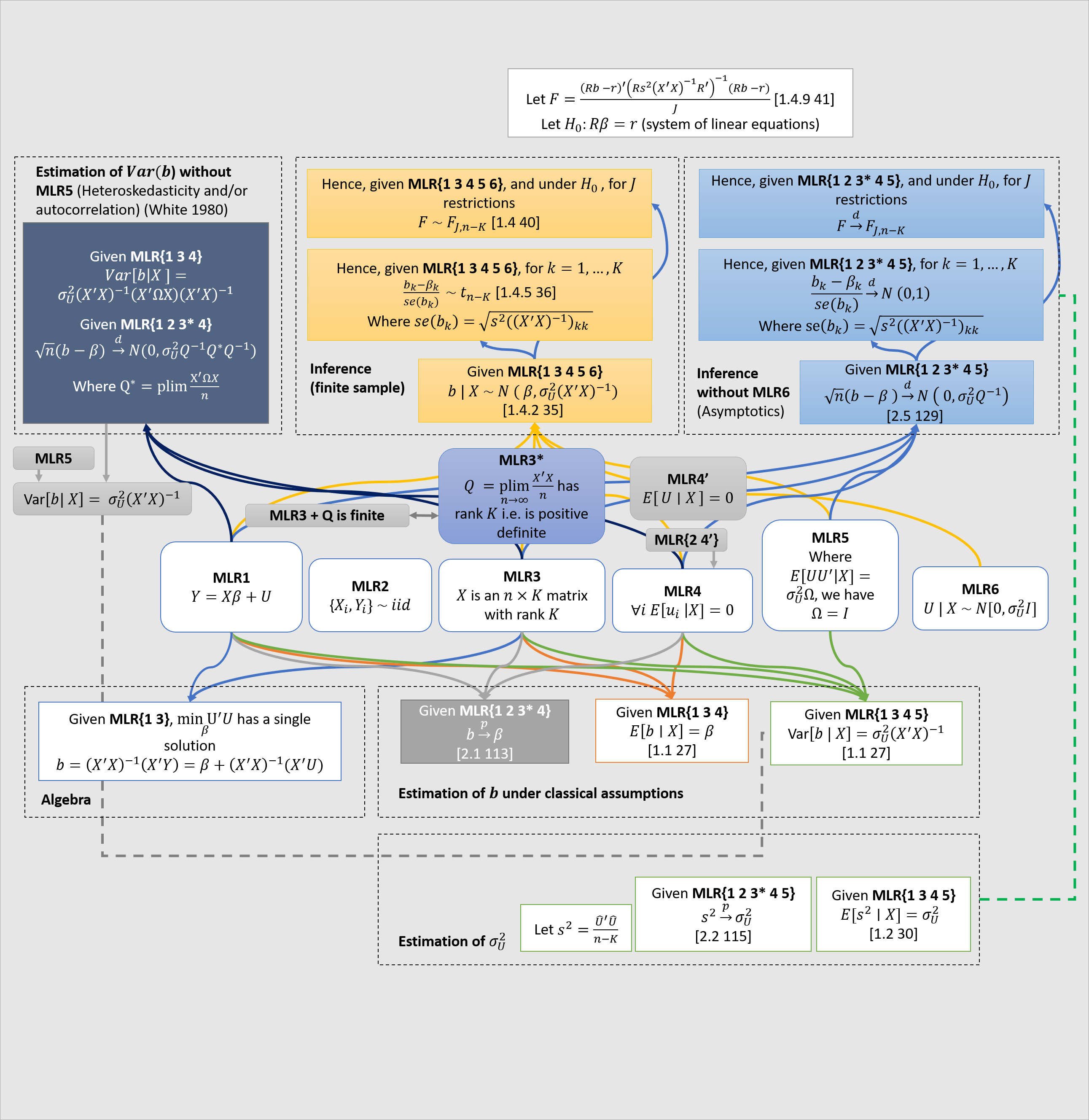
A couple of comments about the diagram are in order.

$U$ , $Y$ are a $n \times 1$ vectors of random variables. $X$ may contain numbers or random variables. $\beta$ is a $K \times 1$ vector of numbers.
We measure: realisations of $Y$ , (realisations of) $X$ . We do not measure: $\beta$ , $U$ . We have one equation and two unknowns: we need additional assumptions on $U$ .
We make a set of assumptions (MLR1-6) about the joint distribution $f(U,X)$ . These assumptions imply some theorems relating the distribution of $b$ and the distribution of $\beta$ .
In the diagram, I stick to the brute mathematics, which is entirely independent of its (causal) interpretation.¹
Note the difference between MLR4 and MLR4’. The point of using the stronger MLR4 is that, in some cases, provided MLR4, MLR2 is not needed. To prove unbiasedness, we don’t need MLR2. For finite sample inference, we also don’t need MLR2. But whenever the law of large numbers is involved, we do need MLR2 as a standalone condition. Note also that, since MLR2 and MLR4’ together imply MLR4, clearly MLR2 and MLR4 are never both needed. But I follow standard practise (e.g. Hayashi) in including them both, for example in the asymptotic inference theorems.
Note that since $X’X$ is a symmetric square matrix, $Q$ has full rank $K$ iff $Q$ is positive definite; these are equivalent statements (see Wooldridge 2010 p. 57). Furthermore, if $X$ has full rank $K$ , then $X’X$ has full rank $K$ , so MLR3* is equivalent to MLR3 plus the fact that $Q$ is finite (i.e actually converges).
Note that given MLR2 and the law of large numbers, $Q$ could alternatively be written $E[X’X]$
Note that whenever I write a $p\lim$ and set it equal to some matrix, I am assuming the matrix is finite. Some treatments will explicitly say $Q$ is finite, but I omit this.
Note that by the magic of matrix inversion, $((X'X)^{-1})_{kk} = \frac{1}{\sum_{i=1}^n (x_{ki} - \bar x _{k})^2}$ . ²
Note that these expressions are equal: $\frac{b_k -\beta_k}{se(b_k)} = \frac{(b_k - \beta_k)\sqrt{n-K}} {\hat{U'} \hat{U} ((X'X)^{-1})_{kk}}$ . Seeing this helps with intuition.

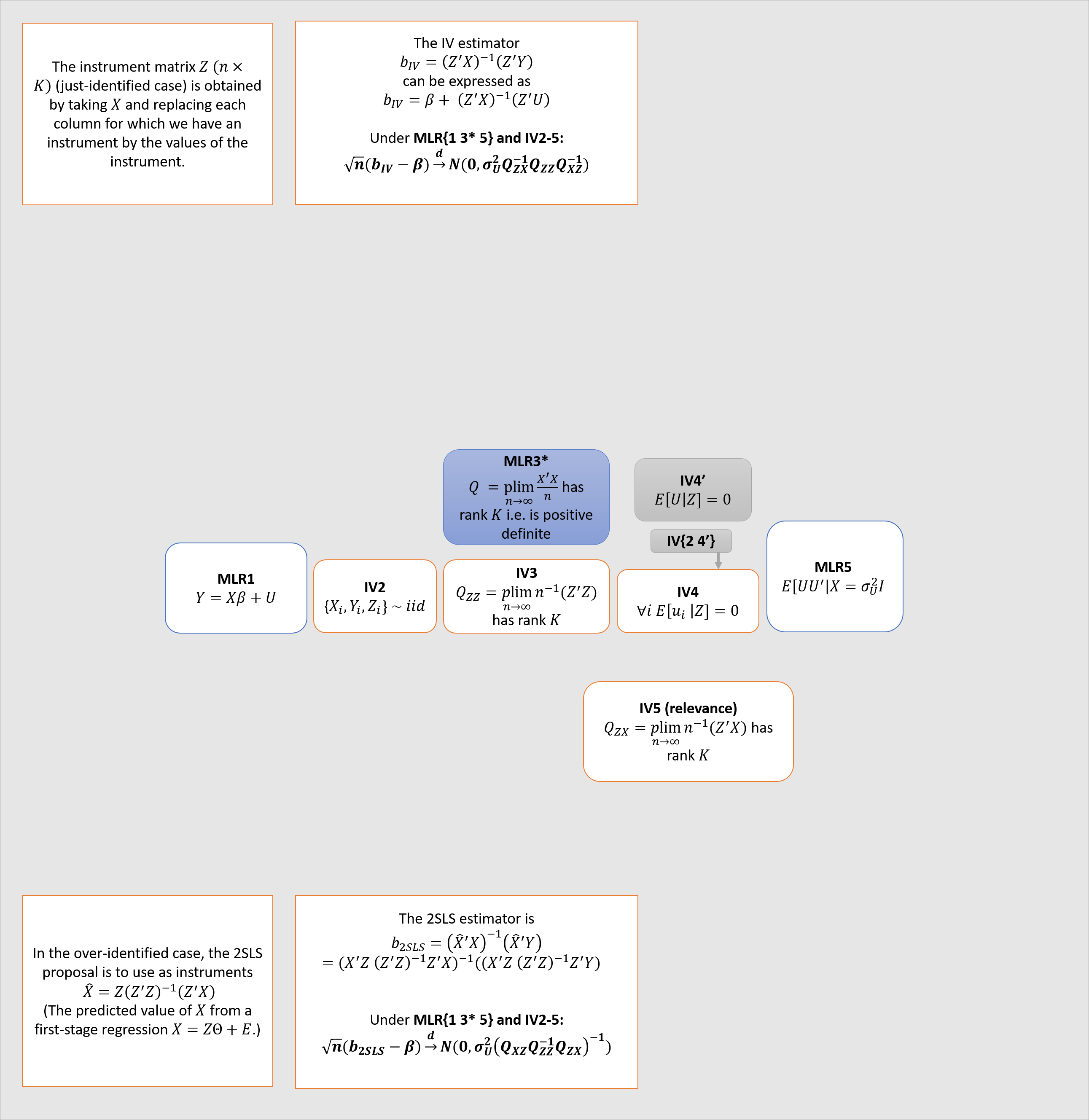
The second diagram gives the asymptotic distribution of the IV and 2SLS estimators.³

I made this is PowerPoint, not knowing how to do it better. Here is the file.

But of course what really matters is the causal interpretation.

As Pearl (2009) writes, “behind every causal claim there must lie some causal assumption that is not discernible from the joint distribution and, hence, not testable in observational studies”. If we wish to interpret $\beta$ (and hence $b$ ) causally, we must interpret MLR4 causally; it becomes a (strong) causal assumption.

As far as I can tell, when econometricians give a causal interpretation it is typically done thus (they are rarely explicit about it):
- MLR1 holds in every possible world (alternatively: it specifies not just actual, but all potential outcomes), hence $U$ is unobservable even in principle.
- yet we make assumption MLR4 about $U$
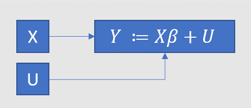
This talk of the distribution of a fundamentally unobservable “variable” is a confusing device. Pearl’s method is more explicit: replace MLR $\{1 \quad 4\}$ with the causal graph below, where $:=$ is used to make it extra clear that the causation only runs one way. MLR1 corresponds to the expression for $Y$ (and, redundantly, the two arrows towards $Y$ ), MLR4 corresponds to the absence of arrows connecting $X$ and $U$ . We thus avoid “hiding causal assumptions under the guise of latent variables” (Pearl). (Because of the confusing device, econometricians, to put it kindly, don’t always sharply distinguish the mathematics of the diagram from its (causal) interpretation.)

↩
Think about it! This seems intuitive when you don’t think about it, mysterious when you think about it a little, and presumably becomes obvious again if you really understand matrix algebra. I haven’t reached the third stage. ↩
For IV, it’s even clearer that the only reason to care is the causal interpretation. But I follow good econometrics practice and make only mathematical claims. ↩

January 10, 2018