Valerio Filoso (2013) writes:

Most econometrics textbooks limit themselves to providing the formula for the $\beta$ vector of the type

$$\beta = (X′X)^{-1} X'Y.$$

Although compact and easy to remember, this formulation is a sort black box, since it hardly reveals anything about what really happens during the estimation of a multivariate OLS model. Furthermore, the link between the $\beta$ and the moments of the data distribution disappear buried in the intricacies of matrix algebra. Luckily, an enlightening interpretation of the $\beta$s in the multivariate case exists and has relevant interpreting power. It was originally formulated more than seventy years ago by Frisch and Waugh (1933), revived by Lovell (1963), and recently brought to a new life by Angrist and Pischke (2009) under the catchy phrase regression anatomy. According to this result, given a model with K independent variables, the coefficient $\beta$ for the k-th variable can be written as

$$\beta_k = \frac{cov(y,\tilde{x}_k)}{var(\tilde x_k)}$$

where $\tilde x_k$ is the residual obtained by regressing $x_k$ on all remaining $K − 1$ independent variables.

The result is striking since it establishes the possibility of breaking a multivariate model with $K$ independent variables into $K$ bivariate models and also sheds light into the machinery of multivariate OLS. This property of OLS does not depend on the underlying Data Generating Process or on its causal interpretation: it is a mechanical property of the estimator which holds because of the algebra behind it.

From, $\beta_k = \frac{cov(y,\tilde{x}_k)}{var(\tilde x_k)}$, it’s easy to also show that

I’ll stick to the first expression in what follows. (See Filoso sections 2-4 for a discussion of the two options. The second is the Frisch-Waugh-Lovell theorem, the first is what Angrist and Pischke call regression anatomy).

Multiple regression with $K\geq3$ (a constant and two or more variables) can feel a bit like voodoo at first. It is shrouded in phrases like “holding constant the effect of”, “controlling for”, which are veiled metaphors for the underlying mathematics. In particular, it’s hard to see what “holding constant” has to do with minimising a loss function. On the other hand, a simple $K=2$ regression has an appealingly intuitive 2D graphical representation, and the coefficients are ratios of familiar covariances.

This is why it’s nice that you can break a model with $K$ variables into $K$ bivariate models involving the residuals $\tilde x_k$. This is easiest to see in a model with $K=3$: $\tilde x_k$ is the residual from a simple $K=2$ regression. Hence a sequence of three simple regressions is sufficient to obtain the exact coefficients of the $K=3$ regression (see figure 2 below, yellow boxes).

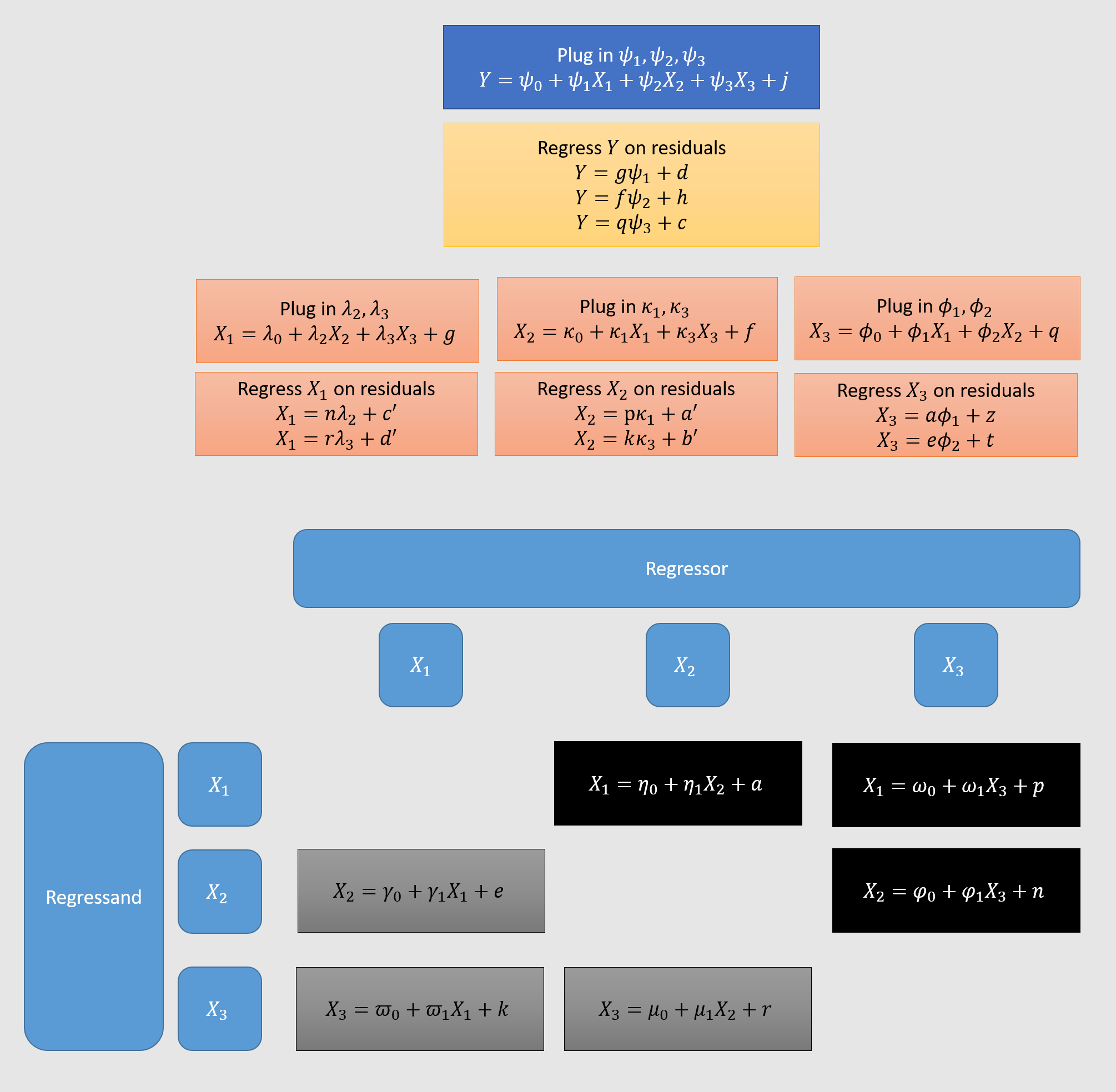
Similarly, it’s possible to arrive at the coefficients of a $K>3$ regression by starting with only simple pairwise regressions of the original $K$ independent variables. I do this for $K=4$ in figure 1. From these pairwise regressions (in black and grey¹), we work our way up to three $K=3$ regressions of one $X$-variable on the two others (orange boxes), by regressing each $X$-variable on the residuals obtained in the first step. We obtain expressions for each of the $\tilde x_k$, ($g,f,q$ in my notation). We regress $Y$ on these (yellow box). Figure 1 also nicely shows that the number of pairwise regressions needed to compute multivariate regression coefficients grows with the square of $K$. According to this StackExchange answer, the total time complexity is $O(K^2n)$, for $n$ observations.

Figure 1:

Judd et al. (2017) have a nice detailed walk-through of the $K=3$ case, pp.107-116. Unfortunately, they use the more complicated Frisch-Waugh-Lovell theorem method of regressing residuals on residuals. I show this method here (in green) and the method we’ve been using (in yellow), for $K=3$. As you can see, the former method needs two superfluous base-level regressions (in dark blue). But they should be equivalent, hence I use the same $\theta$ coefficients in the yellow and green boxes.

Figure 2:

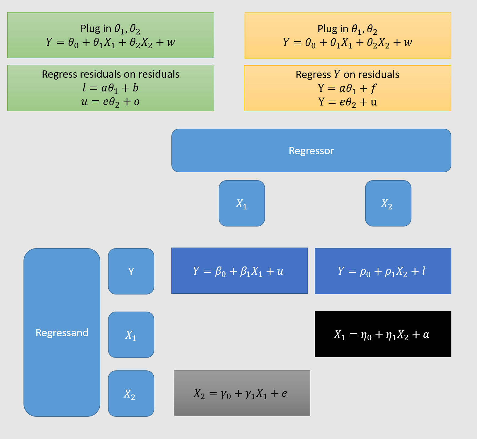
I made this is PowerPoint, not knowing how to do it better. Here is the file.