Suppose a study comes out about the effect of a new medication and you want to precisely compute how to update your beliefs given this new evidence. You might use Bayes’ theorem for continuous distributions.

The normalization constant (the denominator of the formula) is an integral that is not too difficult to compute, as long as the distributions are one-dimensional.

For example, with:

from scipy import stats
from scipy import integrate

prior = stats.lognorm(scale=math.exp(1),s=1)
likelihood = stats.norm(loc=5,scale=20)
def unnormalized_posterior_pdf(x):
	return prior.pdf(x)*likelihood.pdf(x)
normalization_constant = integrate.quad(
    unnormalized_posterior_pdf,-np.inf,np.inf)[0]

the integration runs in less than 100 milliseconds on my machine. So we can get a PDF for an arbitrary 1-dimensional posterior very easily.

But taking a single sample from the (normalized) distribution takes about a second:

# Normalize unnormalized_posterior_pdf
# using the method above and return the posterior as a
# scipy.stats.rv_continuous object.
# This takes about 100 ms
posterior = update(prior,likelihood) 

# Take 1 random sample, this takes about 1 s
posterior.rvs(size=1) 

And this difference can be even starker for higher-variance posteriors (with s=4 in the lognormal prior, I get 250 ms for the normalization constant and almost 10 seconds for 1 random sample).

For a generic continuous random variable, rvs uses inverse transform sampling. It first generates a random number from the uniform distribution between 0 and 1, then passes this number to ppf, the percent point function, or more commonly quantile function, of the distribution. This function is the inverse of the CDF. For a given percentile, it tells you what value corresponds to that percentile of the distribution. Randomly selecting a percentile $x$ and evaluating the $x$ th percentile of the distribution is equivalent to randomly sampling from the distribution.

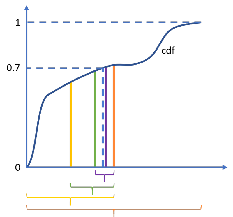
How is ppf evaluated? The CDF, which in general (and in fact most of the time¹) has no explicit expression at all, is inverted by numerical equation solving, also known as root finding. For example, evaluating ppf(0.7) is equivalent to solving cdf(x)-0.7=0, which can be done with numerical methods. The simplest such method is the bisection algorithm, but more efficient ones have been developed (ppf uses Brent’s method). The interesting thing for the purposes of runtime is that the root finding algorithm must repeatedly call cdf in order to narrow in on the solution. Each call to cdf means an expensive integration of the PDF.

The bisection algorithm to solve cdf(x)-0.7=0

An interesting corollary is that getting one random number is just as expensive as computing a chosen percentile of the distribution using ppf (assuming that drawing a random number between 0 and 1 takes negligible time). For approximately the cost of 10 random numbers, you could characterize the distribution by its deciles.

On the other hand, sampling from a distribution whose family is known (like the lognormal) is extremely fast with rvs. I’m getting 10,000 samples in a millisecond (prior.rvs(size=10000)). This is not because there exists an analytical expression for its inverse CDF, but because there are very efficient algorithms² for sampling from these specific distributions³.

So far I have only spoken about 1-dimensional distributions. The difficulty of computing the normalization constant in multiple dimensions is often given as a reason for using numerical approximation methods like Markov chain Monte Carlo (MCMC). For example, here:

Although in low dimension [the normalization constant] can be computed without too much difficulties, it can become intractable in higher dimensions. In this last case, the exact computation of the posterior distribution is practically infeasible and some approximation techniques have to be used […]. Among the approaches that are the most used to overcome these difficulties we find Markov Chain Monte Carlo and Variational Inference methods.

However, the difficulty of sampling from a posterior distribution that isn’t in a familiar family could be a reason to use such techniques even in the one-dimensional case. This is true despite the fact that we can easily get an analytic expression for the PDF of the posterior.

For example, with the MCMC package emcee, I’m able to get 10,000 samples from the posterior in 8 seconds, less than a millisecond per sample and a 1,000x improvement over rvs!

ndim, nwalkers, nruns = 1, 20, 500

start = time.time()
def log_prob(x):
    if posterior.pdf(x)>0:
        return math.log(posterior.pdf(x))
    else:
        return -np.inf
sampler = emcee.EnsembleSampler(nwalkers, 1, log_prob)
sampler.run_mcmc(p0, nruns) #p0 are the starting samples

These samples will only be drawn from a distribution approximating the posterior, whereas rvs is as precise as SciPy’s root finding and integration algorithms. However, I think there are MCMC algorithms out there that converge very well.

Here’s the code for running the timings on your machine.