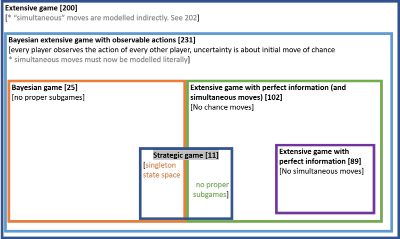
The basic notion of strategic game can be extended in two directions: adding imperfect information, and adding sequential moves. This gives nice matryoshka dolls of types of games, depicted below with page numbers in Osborne and Rubinstein (OR) in brackets.

Each type of game has a solution concept that is arguably natural to it.

Applying the solution concept of a more general game to a more specific game can always be done, but it is uninteresting. For example, all Nash equilibria of a strategic game are trivially subgame perfect, and trivially Bayesian.

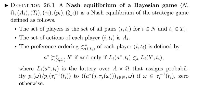
We can also apply the solution concept of a more specific game to a more general game, for example, we can find the Nash equilibria of a game with sequential moves; some of these will not be subgame perfect. Suppose we wanted to do the same thing with Bayesian games. I found that this does not work straight out of the box when using the definitions from OR and other standard textbooks. We will need to make some small changes. In 26.1, OR make the following definition¹:

A Nash equilibrium of a Bayesian game with vNM preferences $\langle N, \Omega,(A_i), (T_i), (s_i), (p_i), (u_i) \rangle$ is a Nash Equilibrium of the strategic game with vNM preferences defined as follows:

• The set of players is the set of all pairs $(i,t_i)$ for $i \in N$ and $t_i \in T_i$

• For each player $(i,t_i)$, the set of actions is $A_i$

• For each player $(i,t_i)$, the preference function assigns to action $a_i$ the payoff

$$\sum_{\omega \in \Omega} p_i(\omega \mid t_i )u_i [(a_i,\hat{a}_{-i}(\omega)), \omega ]$$

where $\hat{a}_{-i}(\omega)$ is the profile of actions taken by every player $(j,s_j(\omega)), j \neq i$ in state $\omega$.

.

For the purpose of seeing the relationships between solution concepts, calling this a “Nash equilibrium” is unfortunate. When we introduce extensive games, we give a new name, “subgame perfect equilibrium” to its natural solution concept. So why re-use the name “Nash equilibrium” for the solution concept of Bayesian games? It would be preferable to call 26.1 a Bayesian-Nash equilibrium of a Bayesian game, as distinct from a Nash equilibrium of a Bayesian game in which the players do not condition on their type. That is, in what I propose to call a Nash equilibrium of a Bayesian game, players choose an unconditional strategy, and their utilities correspond to the expected utilities using their prior over types. Picture the players before they receive their signals. They have some prior over the signals they and their opponents will receive. They can average over this uncertainty and decide on a strategy. If these unconditional strategies are best responses to each other, we have a Nash equilibrium. On this definition, a Nash equilibrium of a Bayesian game ignores all the properly Bayesian features of the game, just like a Nash equilibrium of a sequential game ignores all the sequential information. Why wouldn’t you condition on your type? You would if you were rational! But if you were rational you would also never play a non-subgame perfect Nash equilibrium strategy. Yet we still find it useful to have the specific name “subgame perfect equilibrium of an extensive game”.

Given these definitions, we can find:

• the Bayesian Nash equilibria of a Bayesian extensive game with observable actions; some of these will not be subgame perfect.
• the perfect Bayesian equilibria of an extensive game; in some of these the off-equilibrium-path beliefs will not be consistent [Lecture 8]
• the Nash equilibria of a Bayesian game; some of these will be such that some player-types, if they did condition on their type, would not be best-responding.
• and so on

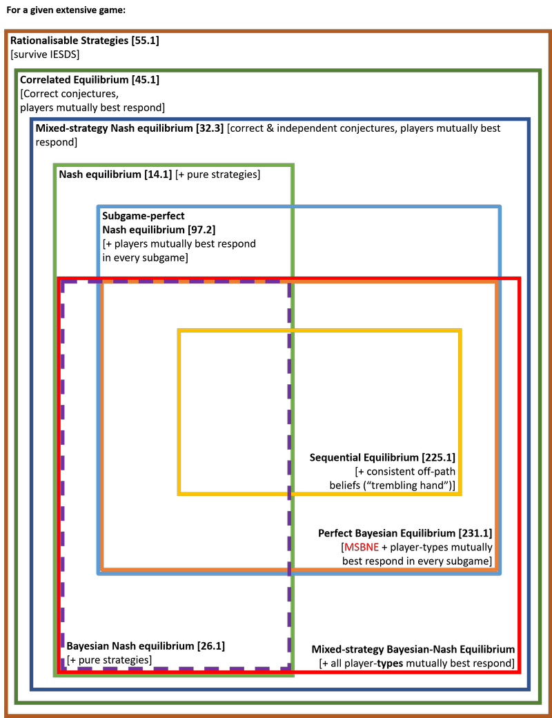
This gives us this diagram:

Notice that we really could not have put all the solution concepts on one diagram if we had been using the standard definition. It would not make sense to speak of the Nash equilibria of a general extensive game, as a proper superset of its Bayesian-Nash equilibria. We would have needed two separate diagrams, one for games of imperfect information, and one for games of perfect information.

Here are some sources for the claims in the second diagram:

• By proposition 45.3, the set of correlated equilibria of G contains the set of mixed strategy Nash equilibria of G.
• By definition 32.3 of a mixed strategy Nash equilibrium, the set of mixed strategy Nash equilibria of G contains the set of Nash equilibria of G.
• Lemma 56.2 states that every strategy used with positive probability by some player in a correlated equilibrium of a finite strategic game is rationalisable.

I used the spaced repetition app Anki to memorise material for PPE finals at Oxford. You can download them below. The quality varies a lot, and the formatting is inconsistent. Many of the cards are heavily customised for my use, and you may not find them helpful. Please also beware that these cards likely contain important errors. Some were reviewed only a few times so I wouldn’t necessarily have caught all mistakes. My guess would be that on the order of 3% of cards contain a substantial error. If despite all this you still want to try them, here you go:

• FHS102 Knowledge and Reality
• FHS103 Ethics
• FHS127 Philosophical Logic and Philosophical Logic proof toolkit
• FHS300 Quantitative economics
• FHS301 Macroeconomics
• FHS302 Microeconomics
• FHS314 Econometrics
• FHS319 Game theory

PPE finals are eight high-stakes examinations on two years’ worth of material, composed of eight modules. Everyone dedicates at least their last term to revision, during which no new modules are added. Many PPE students even finish their eight modules two terms before exams (at the end of Michaelmas term of their third year), which theoretically leaves six months between the time they stop learning new material and the time they are examined.

How much explicit planning should go into finals revision? I am generally wary of over-planning, especially with rigid, brittle plans over long time horizons. The plan often ends up being inadequate, not following the plan causes guilt, and constantly revising it costs a lot of effort¹. On the other hand, when the stakes and the risk of akrasia are both high, planning could have outsize returns.

There are many aspects of planning for exams. Here I focus on just one: budgeting time between different topics for revision. This is especially difficult to do with raw intuition: it always feels like you’ve got ages left until exams, until you don’t. It’s typical for people to take a leisurely stroll through material that they enjoy, deepening their understanding, which leaves little time for the more difficult and aversive stuff. (Given how easily I get nerd-sniped by my favourite topics, this is an especially worrying pitfall for me.)

To budget my time, I used this spreadsheet, which you can copy and adapt². I’ll discuss some of its features now.

Dividing the remaining time

The most basic feature is a simple reality check: how many days until exams? (This is calculated dynamically using =TODAY().) Dividing by eight, how many per module? This simple calculation could be enough to snap you out of the vague feeling that there is “a lot” of time left. Maybe there really is ample time. Why not find out exactly how much, so you can use it best? Maybe once you do the maths you realise there isn’t. In that case this simple division provides a salutary wake-up call.

Further adjustments could be useful. I’d recommend planning some days off, like one day a week, and certainly a few full days before exams (cramming is counter-productive). If you’re travelling or doing any projects, subtract those days explicitly from the total.

If your modules have themselves a modular structure, like independent chapters of a textbook, you might consider further subdividing the time between them. Maybe you’ll get something like 0.12 days per chapter, which at five hours a day is 36 minutes, something so close to the skin your system 1 might actually be able to process it. In my experience it’s pretty rare for intellectual material to actually have such independent chunks, when you zoom in all the way, even though it might superficially be organised into discrete topics.

Allocating time between modules in proportion to their variance

If you’re trying to maximise your expected mark, allocating more time to higher-variance papers makes sense. To be precise, if your mark in each paper is the square root of time allocated times the standard deviation, the sum of the marks is maximised by allocating time in proportion to the variance.

I looked up the variance in marks for each paper since 2015, the first year this information was available in the PPE examiner’s reports. I then averaged the three variances³ for each paper. For a PPE student taking my eight papers, I computed how much of the total variance has historically been contributed by each paper.

The results are pretty striking. For example Game Theory contributed more than four times as much variance as Knowledge and Reality. I think these fractions are a better starting point for time budgeting than allocating time equally between the modules.

But allocating time purely by the variance has some pretty obvious flaws. For starters, there are strong selection effects: some papers are mandatory for everyone, while others select for the most capable and interested students. For instance, if all but the nerdiest of nerds avoid econometrics, we should expect the variance to be artificially low for that paper. Then there is the fact that some modules build on each other while others do not: econometrics is basically an advanced version of quantitative economics, so there is little point doing quantitative economics-specific revision over and above what I do for econometrics. And finally you need to adjust for factors idiosyncratic to you: I basically snoozed through Macroeconomics last year while I was busy with an unrelated research project. I ended up with these target allocations:

Planning for humans: built-in updating

A crucial feature of a good revision plan is that it adapts gracefully when you don’t get as much done as you hoped. You shouldn’t have to scramble to adjust your plan after the fact, cursing your weakness of will. It should be baked into the design from the start.

On one view of plans, they are what you should do, and a feeling of guilt when you don’t follow them is not only natural but appropriate. A view that I’ve often found more fruitful is to treat plans as just another tool of instrumental rationality. This may seem like an obvious point, but for many people, myself included, it’s much harder to grasp on an intuitive level, and harder still to implement. On this topic I highly recommend reading Nate Soares’ replacing guilt series.

When you fall behind your initial plan, it can be tempting to think you can accelerate to make up for lost time. But I think this is rarely realistic. When you don’t work as hard as you had planned, this constitutes evidence that your plan is too ambitious for the future as well as the past. I have often ignored this evidence and paid the price for it. Accelerating is an especially bad idea when you need to allocate your effort over weeks rather than days or hours. Like many beginning endurance runners, if you run that fast you’ll end up collapsing before the finish line.

I used the Pomodoro technique: 25-minute segments of focused work followed by a five-minute break. Apart from its other benefits, this technique provides a nice and tangible unit to measure time. At any point in time I want to be solving this equation:

This graph shows $A_i/S_i$:

Where $P$ is the number of pomodoros left until exams, $S_i$ is the number of pomodoros spent on module $i$ so far, $T_i$ is the overall target allocation for module $i$, and $A_i$ is the allocation (out of $P$) to now be spent on module $i$. For this, I need to manually keep track of an additional variable, $S_i$. I do this on Sheet2.

We can do interesting things with $P$. The simplest estimate of $P$ is simply a constant number of pomodoros times the number of days left until exams (running the entire marathon at the same speed). This is sufficient to give you the first feature of the equation: automatic adjustment to the passing of time.

Tracking $S_i$ enables a second nice feature. By computing your average number of pomos per day ($\sum_i S_i$ divided by the number of days since you started revising), and extrapolating it, you obtain a realistic estimate of $P$. This gives you automatic adjustment for your actual capacity to do work. You needn’t slavishly extrapolate this average. But it should feed into your estimate of $P$. If you plan to work 10 pomos a day but so far you’ve only done an average of 4 pomos a day, that should raise a red flag.

Diminishing returns suggest that it’s best to always work on the module for which $T_i/S_i$ (depicted below) is largest.

The budget as a part of a larger decision-making procedure

I often disregarded the numbers based on hunches and intuitions, especially when I felt that my intuitions were capturing some unmodeled factor (for instance when I felt confident about a topic without having spent much time revising it, or when I postponed revision on exams which came later).

I fully expected that I would do this. Getting up every day and following the dictates of the spreadsheet would have been an instance of Spock-like “straw vulcan” rationality. Instead, I viewed the model and the intuitive view as two different tools at my disposal, or as two advisors, each with her own bias.

I thought of the division of labour in something like the following way. The whole case for making an explicit, numerical budget is that the intuitive System 1 is about as good at long-term planning as a toddler in a casino. The spreadsheet is excellent at remembering what you did, keeping track of the long-term goals, feeding historical data into your decision making process, and most importantly, it does not self-delude. However, it is a woefully simplified model of the actual task of taking eight exams while trapped in a human body with a fleshy brain. Millions of variables are boiled down to a handful. The model is computationally puny next to the awesome power of your System 1, whose inclinations are based on a great deal of contextual information which your brain constantly gobbles up. System 1 shines at taking in a huge amount of relevant information and boiling it down to an up-or-down judgement: Game Theory today, yea or nay? The spreadsheet is good at correcting some of the biases of System 1 and at giving enough weight to the data on variances, which is crucial but not at all salient.

How useful was all this planning?

Looking back, how much did the budget actually change my decisions? I ended up using the model mostly as a guardrail, reminding me to allocate more time to a module when its ratio $A_i/S_i$ became something outrageous like 300%. I didn’t pay much attention to the exact numbers on a day-to-day basis. But averaging over the long run, I think the budget substantially affected my decisions. In particular, it made me spend much less time on low-variance philosophy papers and more on game theory and microeconomics.

Another intended purpose of the spreadsheet was to help me smooth my effort more over time. Looking back, I’m a bit disappointed by how much harder I worked when finals were approaching than when they were more distant. But it probably would have been even worse with less planning. My best guess is that the spreadsheet had a minor positive impact in this respect. To be fair, effort and consumption smoothing is, in general, a very difficult task for human motivation.

My final allocations turned out to be pretty close to the targets even though I didn’t strongly intend them to.

Given the high stakes and the relatively low time cost, I think this project was amply worth it. Setting up the spreadsheet took only a few hours. The main cost was the hassle of keeping track of daily time use. The single biggest win was to do the research on the variances. For this insight I thank my friend Rune Tybirk Kvist, who completed finals one year before me.