In the UK, many internet service providers (ISPs) block Sci-Hub. However, a simple proxy is enough to circumvent this (you don’t even need a VPN). Routing requests through a suitable1 proxy lets you open Sci-Hub in your regular browser as if it weren’t blocked2.
Routing all your traffic through a proxy may come with privacy and security concerns, and will slow your connection a bit. We want to use our proxy only for accessing Sci-Hub.
You can use extensions like ProxySwitchy to tell your browser to automatically use certain proxies, or no proxy at all, for sets of websites that you define.
Unfortunately, this extension, and others like it, require permissions to insert arbitrary JavaScript into any page you visit (the web store accurately explains that the extension can “read and change all your data on the websites you visit”). That’s likely due to insufficiently granular permission definitions by Chrome, and is not the fault of the presumably well-intentioned extension authors. But it freaks me out a little bit (bad things have happened).
Luckily, we can achieve the same effect by writing our own proxy auto-configuration file. A proxy auto-configuration or PAC file contains just a single JavaScript function like this:
functionFindProxyForURL(url,host){// Sci-Hub requestsif(shExpMatch(host,'sci-hub.se')||shExpMatch(host,'*.sci-hub.se')){// Your proxy address and port numberreturn'PROXY 123.456.789:9279';}// All other requestsreturn'DIRECT';}
We can instruct the operating system to read this file. Search for instructions on Google (example).
When you use the proxy to access Sci-Hub for the first time in a browser session, the browser will ask you for the username and password to your proxy server. If you’re using Chrome, I’d recommend saving the credentials into the browser’s password manager to avoid having to enter them again.3
There are many free proxies on the Internet, but I find that using the services of an actual for-profit proxy company is well worth it, for the greater speed and reliability. Currently webshare.io (referral link) offers 1 GB per month free, which is quite a lot of Sci-Hub PDFs. After that you can get 250 GB for $2.99 per month.4
Choose a proxy from your list, and copy its address and port number into your PAC file, following the pattern above.
Set your operating system to read its proxy settings from this PAC file5. Instructions for this are easy to Google (example).
Open Sci-Hub in your browser. Enter your proxy username and password and optionally save these credentials in the browser. You can find the credentials in your webshare.io account.
Don’t forget to only use Sci-Hub to look at really old papers that have lapsed into the public domain :)
Obviously, the proxy must not itself be on a network that blocks Sci-Hub. I have not come across any proxy that blocks Sci-Hub in this way. ↩
Changing your DNS resolver to a public one like Google’s instead of your ISP’s is not sufficient as of 2021, for two ISPs I’ve tested, and I suspect for all UK ISPs that implement blocking. (Many people believe changing the DNS resolver is sufficient. Probably ISPs used to implement simple DNS level blocking and have recently upped their game.) My guess is that instead of merely blocking the request to resolve sci-hub.se at the DNS resolver level, the ISPs are also doing a reverse lookup on every requested IP address to check whether it corresponds to a blacklisted domain. ↩
You want to use the Chrome password manager because third-party password managers such as 1Password are not able to auto-fill credentials when logging in to a proxy server (as opposed to logging into a webpage). Note that if you have a third-party password manager extension installed this will disable the browser setting “Offer to save passwords”. I recommend that you temporarily disable your password manager extension, log in to your proxy server, save the password into Chrome, and then enable the extension again. ↩
Their home page exemplifies a dark pattern by not showing the pricing by the GB; it just says you get ‘up to unlimited’ bandwidth. You’ll be able to see the actual pricing after you create an account. ↩
One gotcha is that Windows 10 forces you to call your PAC file from a web server; it cannot be a local file (??!). To work around this, you can upload your file as a Gist and link to the /raw. ↩
Summary:I have tried many types of masks and respirators during the 2020 pandemic. My recommendation is to use ‘elastomeric’ respirators common in industry, and to either filter or completely block off their exhalation valve. The result is a comfortable respirator that I believe offers a high level of protection against airborne diseases to myself and others. I am not an infectious disease expert.
The effectiveness of a mask can be broken down into two parts: how well the mask fits on your face, and the filtration efficiency of the mask. A further important consideration is comfort.
Surgical and cloth masks are comfortable but have poor fit and filtration efficiency. I believe it’s possible to do much better.
Respirators that meet the NIOSH N95 or N99 standards for filtration efficiency, such as the N95 respirators pictured below, are popular in healthcare settings.
3M N95 respirator (left), N95 respirator in a medical setting (right)
In my experience, these have two main downsides:
They may be scarce during pandemics. You should probably leave limited supplies for healthcare workers.
The tight elastic band that ensures a good fit also makes the respirators very uncomfortable for extended use.
KN95 and KF95 are respectively the Chinese and Korean-manufactured masks that claim to have the same efficacy as N95s. They come with ear loops rather than behind-the-head elastic bands, so they have a far looser seal than N95s. I suppose you could add your own elastic bands to them to improve the seal, but then they would be just as uncomfortable as N95s. Therefore, they are not a competitive option.
A KN95 mask
There also exist N95+ masks designed for industrial tasks that produce harmful airborne particles (such as welding or paint spraying). They are called elastomeric respirators, or sometimes industrial respirators.
High filtration efficiency elastomeric respirators for industrial use. Miller LPR-100 (left), 3M 6200 (right).
Compared to healthcare N95s, these respirators:
are more widely available
achieve superior fit by using elastomers shaped like a human face (there is no need to bend a metal nose bridge)
are much more comfortable, mainly because they:
spread the pressure onto a wider area of skin
come in multiple sizes
have adjustable straps
won’t fog up your glasses
A downside is that it’s more difficult to be audible through an elastomeric respirator than through an N95 or surgical mask. I am able to be understood by raising my voice, but smooth social interactions are not guaranteed. It’s probably not a great setup for spending time with your friends; you can use a KN95 for that.
The fatal flaw1 of these elastomerics when it comes to disease control is that they have an exhalation valve that allows unfiltered air to exit the mask. In PPE jargon, they do not provide source control. (This may be about to change in 2021, see this footnote2. I will try to keep this post updated.)
The exhalation valve opening on the Miller LPR-100
We can modify these respirators to filter their exhalation valve (recommendaton A), or completely close it off (recommendation B).
(If infection through the mucosal lining of the eyes is an important concern to you, and you don’t wear glasses, you should also wear safety googgles.)
CDC recommendation for exhalation valves
During the 2020 pandemic, the US CDC issued the following recommendation, in a blog post from August 8 20203:
If only a respirator with an exhalation valve is available and source control is needed, cover the exhalation valve with a surgical mask, procedure mask, or a cloth face covering that does not interfere with the respirator fit.
Recommendation A: 3M 6500QL Series with KN95 and surgical mask
If you want to follow something similar to CDC guidance, I recommend:
A part of a KN95/KF95 mask tightly covering the exhalation valve
3M 6502QL. Unmodified (left), KN95 material covering valve (middle and right)
You’ll likely want to add a surgical mask on top of that:
as a backup
for the very small amount of additional filtration it provides
to avoid misunderstandings with strangers
3M 6502QL with KN95 material covering valve and a surgical mask on top
Surgical masks are not primarily designed to filter aerosols4. It seems clear to me that KN95s and KF95s are superior to a surgical mask for covering an exhalation valve (let a alone a cloth mask). (There is a list of such respirators that have received an emergency use authorization from the FDA. There are probably many low-quality masks fraudulently marketed as KN95 and KF95 at the moment, so make sure you buy from an approved manufacturer.)
In the models I have seen, the material in KN95s is far more flexible than in N95s, making allowing you to shape it so that it tightly covers an exhalation valve. It’s slightly fiddly but definitely possible with a bit of dexterity and perseverance. Using a thinner surgical mask would be easier; but the KN95’s extra protection for third parties is well worth it.
Here are the steps you should follow (see video):
cut a KN95 in half along the fold
cut one half to size further
use a rubber band and tape to attach the material over the respirator valve. This is better explained with a video than in words. The main thing to know is that you should use the two small ridges in the plastic below the valve to secure the rubber band.
add tape on the upper end of the KN95 material
Instructions
Unfortunately, for any valve covering approach, there is a trade-off between a fit and the surface area usable for exhale filtration. I have not been able to achieve a good fit when placing a KN95 or surgical mask more loosely over the valve, which would give more surface area. In my setup a small rectangle of KN95 has to do all the filtration, which likely lowers the efficiency. However, the N95 specification is for a flow rate of 85 liters per minute, which is many times the 6 liters per minute breathed by an individual at rest5, so I am not very concerned.
Ridges on 6502QL. Note that in the real setup the KN95 will go below the elastic band.
Location of the valve underneath the KN95 material. View form below the respirator.
Choice of respirator
I have tried two industrial respirator models, the 3M 6502QL and the Miller LPR-100. I prefer the build quality and aesthetics of the Miller (see below), but its shape makes it almost impossible to get a good seal if you attempt to cover the valve with a surgical mask or KN95. So for this technique, I recommend the 3M 6500QL series.
I am aware of three 3M half-facepiece reusable respirator groups, the 6000 series, the 6500 series, and the 7500 series.
Since I have only tried a respirator of the 6500 series, I do not have a strong view on which is preferable. I would recommend the 6500, mostly because I have already demonstrated that it’s possible to cover the valve. The 6000 series does not have a downward-facing exhalation valve and may be harder to work with. I’m agnostic about the relative merits of the 7500.
The 6500 series has a quick latch version (difference explained here), which is the one I used. I’d recommend the quick latch 6500QL series, because it seems that the latch makes the fit of the KN95 material to the respirator more secure (see video). By the way, attaching a mask on top of the valve makes the quick-latch mechanism much less effective; I never use it.
Each series comes in three sizes, large, medium and small. I am a male with a medium-to-large head, and I use a medium (the 6502QL).
Regarding whether airlines will accept this setup, I have heard both some positive anecdotes and one negative anecdote.
Choice of filters for a 3M respirator
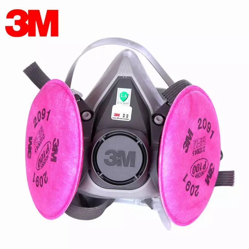
I use the 3M 2097 P100 filters.
You should use lightweight filters that are rated N100, R100 or P100. The “100” means that 99.97% of particles smaller than 0.3 micrometres are filtered out. The letters N, R and P refer to whether the filter is still effective when exposed to oil-based aerosols, this should be irrelevant for our purposes.
The weight of the filters is a crucial determinant of comfort. I originally used the 3M respirator with the 3M 60926 cartridges, which filter gases and vapors as well as particles. This was a mistake, as filtering gases and vapors is irrelevant from the point of view of infectious disease, and these cartridges are much heavier than the 3M 2097 P100 filters. Switching to the lighter filters made a world of difference; now wearing the 3M doesn’t bother me at all.
The 3M 6502QL respirator weighs 395 g. with 3M 60926 cartridges, but only 128 g. with 3M 2097 filters, a 68% reduction.
Recommmendation B: Miller LPR-100 with tape and surgical mask
I believe that, in expectation, the previous method offers slightly worse protection to third parties than a well-fit valveless medical N95, because our makeshift exhalation valve filter may not be entirely effective.
This section details another technique which may be able to achieve the best of both worlds: the comfort and availability of industrial masks, and the third-party protection offered by valveless masks.
How we need to modify the respirator
Let’s look at how the valves in industrial masks work. I’ll be using the Miller LPR-100, but the 3M is built similarly.
The exhalation valve is at the front. There are also two inhalation valves, one on each side between the mouth and the filter. These only allow air to come into the mask from outside, forcing all the exhaled air to go through the exhalation valve (instead of some of it going back through the filter).
Miller LPR-100 valves
We need to disable both the inhalation and exhalation valves:
The unfiltered exhalation valve should be completely sealed off.
In order to allow the user to exhale, the inhalation valves need to be turned into simple holes that allow two-way air circulation.
This will mean that both inhaled and exhaled air will go through the P100 filters.
Exhalation valve
We can seal off the exhalation valve from the outside with tape6. On the Miller respirator, there is a little plastic cage covering the valve, and this cage can be taped over. Note that tape sticks very poorly to the elastomer (the dark blue material on the Miller). This is why I only place tape on the plastic; this seems to be sufficient.
Tape on exhalation cage
I am using painter’s tape because it’s supposed to pull off without leaving a residue of glue. It’s possible that it would be better to use tape with a stronger adhesive. (A friend of mine commented: “Some ideas for sealing off the exhalation valve: (1) Butyl tape/self-vulcanizing tape. Not so much a sticky tape as a ribbon of moldable putty, so no adhesive residue. This stuff is pretty much unparalleled if you need to make a fully gas- and watertight seal around an irregularly shaped opening in a pinch without making a mess. The fact that it has no adhesive does put some constraints on the geometry of the part you’re sealing off, but I think it would work (better than painter’s tape, at least) on the Miller. (2) Vinyl tape/electrical tape. It’s relatively water-resistant and can be stretched to some extent. The adhesive also sticks to polymers pretty well (although it does leave a lot of residue after some time, but you can clean that off with a bit of IPA).”)
You can check the seal of your tape by pressing the mask onto your face and attempting to exhale (with the inhalation valves intact). Air should only be able to escape through the sides of the mask.
Inhalation valves
The inhalation valves are removable and can be pulled out. They are very thin and feel like they might be about to break when you pull them out, but I have been able to pull four of them out without a problem.
Touching a valve (left), a valve after it has been pulled out (right)
The two inhalation valves (left), the filter now visible through the holes (right)
Pushing the valves back in is easy.
The tape can be removed and the valves re-inserted, making my modification fully reversible.
Also use a surgical mask
Even if you’re using the tape technique, I recommend also covering the respirator with a surgical mask, since this has no downsides and might have some benefit. The seal on the exhalation valve might not be perfect and may get worse over time, so an extra layer of filtration, however imperfect, is a good backup.
It’s also beneficial because it makes what you’re doing legible to others. You don’t want to explain this weird tape business to strangers, even if it’s for their protection.
Miller LPR-100. Unmodified (left), with tape (middle), with tape and surgical mask (right)
Since the Miller is better than the 3M, and 3M is such a huge player in this market, I think there’s a decent chance that the Miller is in fact one of the very best options that exists.
The Miller weighs 139 g., which is a negligible difference to the 3M’s 128 g
I also like the fact that you can buy a neat rigid case to hold the Miller respirator. The case is called the 283374.
Miller case, 283374
The Miller model comes with replaceable P100-rated filters, while the 3M can be used with many types of filters and cartridges.
If you want to implement this technique on the 3M, it should be possible; all steps will be similar.
Potential concerns
The 3M+KN95 method we discussed earlier can be seen as a simple adaptation of CDC guidelines, so I have fewer concerns about it.
However, the tape technique involves a more fundamental alteration. This might seem unwise. How do I know I haven’t messed up something crucial, endangering myself and others?
Before discussing the specific concerns, it’s useful to consider: what are the relevant alternatives to my recommendation?
My best guess is that constantly wearing a correctly fitted medical N95, with the really tight elastic bands, is very slightly safer for others in expectation than the tape method (due to risks of things going wrong, like the tape getting unstuck). However, it is not a likely alternative for everyday use. First, in my experience, N95s are more difficult to fit correctly than industrial masks. Second, for me, these respirators are prohibitively uncomfortable. I have seen few people use them. I think the realistic alternatives for most people are cloth and surgical masks. I am relatively confident that both of my techniques are an improvement on that, for both the user and third parties.
By the way, I am not an expert in disease control. I studied economics and philosophy and then worked as a researcher.
Repeated use
Healthcare N95s are supposed to be used only once before being decontaminated. However, I plan to use the same filters many times. Is this a problem?
Why are N95s supposed to be used once? According to this CDC guidance,
the most significant risk [of extended use and reuse] is of contact transmission from touching the surface of the contaminated respirator. … Respiratory pathogens on the respirator surface can potentially be transferred by touch to the wearer’s hands and thus risk causing infection through subsequent touching of the mucous membranes of the face. …
While studies have shown that some respiratory pathogens remain infectious on respirator surfaces for extended periods of time, in microbial transfer [touching the respirator] and reaerosolization [coughing or sneezing through the respirator] studies more than ~99.8% have remained trapped on the respirator after handling or following simulated cough or sneeze.
Since I plan to leave the respirator unused for hours or days between each use, and any viral dose on the exterior of the filters is likely to be very small, I don’t think this is a huge concern overall. I am very open to contrary evidence.
By the way, based on this guidance, it seems to me we should also worry less about reusing respirators and masks in general, even without decontamination. (Decontamination makes a lot more sense for health care workers who are exposed to COVID patients).
It’s good to remember to avoid touching the filters.
CDC guidelines
As explained above, the CDC recommends a surgical or cloth mask to cover the valve. There is no evidence that they considered either of the techniques I described above when issuing their blog post.
The tape method is a greater deviation from the CDC guidelines than the KN95-covering method, so if you care about following official guidance you could use the latter.
Concerns specific to tape method
I assign a relatively low chance that the tape method is worse than the CDC recommendation of covering the valve with a surgical mask (my views depend considerably on the tightness of the surgical mask seal).
and a very low chance that it’s worse than a surgical mask alone. The probability mass I assign to harm is a combination of concerns about exhaling through the filter reducing its efficacy, and unknown unknowns.
C02 rebreathing
Without the valves, part of the air you inhale will be air that you just exhaled, which contains more C02. I have not personally noticed any effects from this.
Exhaling through filter
Could exhaling through the filter be a bad thing somehow? I wasn’t able to find any source making an explicit statement on this, but I think it’s unlikely to be a problem.
One reason to worry is that the founder of Narwall Mask has told me that, according to one filtration expert he spoke to, one-way airflow greatly prolongs the life of the filters compared to two-way airflow. However, based on my small amount of research, I don’t think the life of the filters would be affected to a degree that is practically important.
The MSA valveless elastomeric respirator that I mentioned in this footnote2 appears to have filters that can be used for more than 1 month of daily use during the workday; and moreover, we can see in the respirator’s brochure that these filters, with model number 815369, are the same as those that are used in MSA’s line of regular, valved elastomeric respirators (see here). From this I conclude that: two-way airflow through regular P100 filters was considered an acceptable design choice by MSA; and these filters can be used two-way for at least a month of hospital use.
In addition, healthcare N95s (without valves) are designed to be exhaled through. They are only rated for a day of use, but I believe this is not because the filter loses efficacy (see section on repeated use).
Exhaled air has a relative humidity close to 100%. Could exposure to humid air reduce the efficacy of the filters? In this study of N95 filters, the difference penetration rose from around 2% to around 4% when relative humidity went from 10% to 80%, and this effect increased with duration of continuous use. The flow rate was 85 L/min.
Note that this study, which simulates inhalation of humid air, does not address (except very indirectly) the question of how the exhalation humidity affects the inhalation filtration.
Discussion of tape technique by others
This NIOSH study tested three modifications of valved respirators: covering the valve on the interior with surgical tape, covering the valve on the interior with an electrocardiogram (ECG) pad, and stretching a surgical mask over the exterior of the respirator.
They found that “penetration was 23% for the masked-over mitigation; penetration was 5% for the taped mitigation; penetration was 2% for the [ECG pad] mitigation”. I would be very interested in more discussion of why the ECG pad did so much better than the surgical tape, the authors don’t say much. One guess could be that the ECG pad has a more powerful adhesive, which would suggest that it’s important to choose a strongly adhesive tape if implementing my technique.
When discussing the choice of modification strategies, the authors wrote that “two concerns are that the adhesive could pull away from the surface, thereby not blocking airflow to the same degree over time, and that these adhesives could contain chemicals that have toxicological effects.”
In an FAQ released by 3M, in response to the question of whether one should tape over the exhalation valve, they wrote “3M does not recommend that tape be placed over the exhalation valve”, but do not give any reasons for this beyond the fact that it may become “more difficult to breathe through … if the exhalation valve is taped shut”.
The state of Maine’s Department of Public Safety recommends against tape-covering, but merely because “this would be considered altering the device and violates the manufacturer’s recommendation”.
Overall recommendation
I think it’s about 50/50 which of my two methods is better all things considered. They’re close enough that I think the correct decision depends on how much you care about protecting yourself vs source control. If source control is a minor consideration to you, I’d go with the KN95 valve coverage method, otherwise the tape method.
(As I said in a previous footnote2, if a valveless elastomeric mask is widely available by the time you read this, that is absolutely a superior option to the hacks I have developed.)
(The Narwall Mask is a commercial solution based on a snorkel mask that may be appealing if you don’t mind (i) the lack of NIOSH-approval and (ii) buying from a random startup, and (iii) you don’t mind or even prefer the full-facepiece design.)
Or is it fatal? I had always assumed it was a fatal flaw, until I found some experts arguing otherwise. In this commentary, the authors say: “Data characterizing particle release through exhalation valves are presently lacking; it is our opinion that such release will be limited by the complex path particles must navigate through a valve. We expect that fewer respiratory aerosols escape through the exhalation valve than through and around surgical masks, unrated masks, or cloth face coverings, all of which have much less efficient filters and do not fit closely to the face”.
I have been able to find some data; this recent NIOSH study finds that valved N95s have 1-40% penetration. “some models … had less than 20% penetration even without any mitigation. Other models … had much greater penetration with a median penetration above 40%.” Note that for these tests, the flow rates of 25-85 L/min are higher than the 6 L/min of a person at rest, and that lower flow rates had lower penetration.
Penetration rates of tens of percent are not very good, and not acceptable for my standards, but it’s less bad than I expected, perhaps competitive with surgical masks, and better than cloth masks!
In fact, as of November 25 2020, the company MSA Safety announced in a press release that the first elastomeric respirator without an exhalation valve has been approved by NIOSH. It’s called the Advantage 290 Respirator. The product page has some good documentation.
This journal article from September 2020, although it does not mention MSA, appears to be about the Advantage 290. (This is based on the picture in Fig 1. resembling the picture in the press release, and the fact that the hospitals in the paper are in Pennsylvania and New York states, while MSA is headquartered in Pennsylvania). The article explains how it was rolled out to thousands of healthcare workers (a first wave had 1,840 users). They claim that the cost was “approximately $20 for an elastomeric mask and $10 per cartridge”, which is amazingly low.
They write: “After more than 1 month of usage, we have found that filters have not needed to be changed more frequently than once a month”.
Unfortunately, it seems to be difficult to get one’s hands on one of these right now. The website invites you to contact sales, and the lowest option for “your budget” is “less than $9,999”.
Moreover, even if you were able to get the Advantage 290, it might be too selfish to do so, since this respirator is likely to otherwise be used by healthcare workers. On the other hand, the price signal you create would in expectation lead to greater quantities being produced, partially offsetting the effect. If you are able to get one by paying a large premium over the hospital price, this may even be net positive for others.
If this respirator became available in large quantities, everything I say here would be obsolete.
By the way, I am astonished that it took until this November 2020 for a PPE company to create a valveless elastomeric respirator, this seems to be a very useful product for any infectious disease situation. ↩↩2↩3
It’s unclear to me how much one should downweight this recommendation due to appearing on a CDC blog rather than as more formal CDC guidance. In the post, the recommendations are called “tips”. ↩
The FDA says: “While a surgical mask may be effective in blocking splashes and large-particle droplets, a face mask, by design, does not filter or block very small particles in the air that may be transmitted by coughs, sneezes, or certain medical procedures.” ↩
3M claims that “85 liters per minute (lpm) represents a very high work rate, equivalent to the breathing rate of an individual running at 10 miles an hour”. These lecture notes say that a person has a pulmonary ventilation of 6 L/min at rest, 75 L/min during moderate exercise, and 150L/min during vigorous exercise. ↩
I tried two other methods before I settled on using tape: gluing a thin silicon wafer over the valve on the inside of the mask, and applying glue to the valve directly. Both these methods are entirely inferior and should not be used. ↩
The model number is ML00895 for the M/L size, and ML00894 for the S/M size. ↩
Monadic predicate logic (with identity) is decidable. (See Boolos, Burgess, and Jeffrey 2007, Ch. 21. The result goes back to Löwenheim-Skolem 1915).
How can we write a program to check whether a formula is logically valid (and hence also a theorem)?
First, we have to parse the formula, meaning to convert it form a string into a format that represents its syntax in a machine-readable way. That format is an abstract syntax tree like this:
Formula:
∀x(Ax→(Ax∧Bx))

Abstract syntax tree:
∀
├── x
└── →
    ├── A
    │   └── x
    └── ∧
        ├── A
        │   └── x
        └── B
            └── x
Writing the parser was a fun lesson in a fundamental aspect of computer science. But there was nothing novel about this exercise, and not much interesting to say about it.
The focus of this post, instead, is the part of the program that actually checks whether this syntax tree represents a logically valid formula.
To start with, we might try to evaluate the formula under every possible model of a given size. How big does the model need to be?
We can make use of the Löwenheim-Skolem theorem (looking first at the case without identity):
If a sentence of monadic predicate logic (without identity) is satisfiable, then it has a model of size no greater than 2k, where k is the number of predicates in the sentence. (Lemma 21.8 BBJ).
A sentence’s negation is satisfiable if and only if the sentence is not valid, so the theorem equivalently states: a sentence is valid iff it is true under every model of size no greater than 2k.
For a sentence with k predicates, every constant c in the model is assigned a list of k truth-values, representing for each predicate P whether P(c). We can use itertools to find every possible such list, i.e. every possible assignment to a constant.
The list of every possible assignment to a constant has a length of 2k.
We can then ask itertools to give us, for a model of size m, every possible combination of m such lists of possible constant-assignments. We let m be at most 2k, because of the theorem.
>>>forminrange(1,2**k+1):>>>possible_models=[iforiinitertools.product(possible_predicate_combinations,repeat=m)]>>>print(len(possible_models),"possible models of size",m)>>>formodelinpossible_models:>>>print(list(model))4possiblemodelsofsize1[(True,True)][(True,False)][(False,True)][(False,False)]16possiblemodelsofsize2[(True,True),(True,True)][(True,True),(True,False)][(True,True),(False,True)][(True,True),(False,False)][(True,False),(True,True)][(True,False),(True,False)][(True,False),(False,True)][(True,False),(False,False)][(False,True),(True,True)][(False,True),(True,False)][(False,True),(False,True)][(False,True),(False,False)][(False,False),(True,True)][(False,False),(True,False)][(False,False),(False,True)][(False,False),(False,False)]64possiblemodelsofsize3[(True,True),(True,True),(True,True)][(True,True),(True,True),(True,False)][(True,True),(True,True),(False,True)][(True,True),(True,True),(False,False)][(True,True),(True,False),(True,True)][(True,True),(True,False),(True,False)][(True,True),(True,False),(False,True)][(True,True),(True,False),(False,False)][(True,True),(False,True),(True,True)][(True,True),(False,True),(True,False)]...256possiblemodelsofsize4[(True,True),(True,True),(True,True),(True,True)][(True,True),(True,True),(True,True),(True,False)][(True,True),(True,True),(True,True),(False,True)][(True,True),(True,True),(True,True),(False,False)][(True,True),(True,True),(True,False),(True,True)][(True,True),(True,True),(True,False),(True,False)][(True,True),(True,True),(True,False),(False,True)][(True,True),(True,True),(True,False),(False,False)][(True,True),(True,True),(False,True),(True,True)][(True,True),(True,True),(False,True),(True,False)]...
What’s unfortunate here is that for our k-predicate sentence, we will need to check ∑m=12k(2k)m=2k−12k((2k)2k−1) models. The sum is very roughly equal to its last term, (2k)2k=2k2k. For k=3, this is a number in the billions, for k=4, it’s a number with 19 zeroes.
So checking every model is computationally impossible in practice. Fortunately, we can do better.
Let’s look back at the Löwenheim-Skolem theorem and try to understand why 2k appears in it:
If a sentence of monadic predicate logic (without identity) is satisfiable, then it has a model of size no greater than 2k , where k is the number of predicates in the sentence. (Lemma 21.8 BBJ).
As we’ve seen, 2k is the number of possible combinations of predicates that can be true of a constant in the domain. Visually, this is the number of subsets in a partition of the possibility space:
If a model had a size of, say, 2k+1, one of the subsets in the partition would need to contain more than one element. But this additional element would be superfluous insofar as the truth-value of the sentence is concerned. The partition subset corresponds to a predicate-combination that would already be true with just one element in the subset, and will continue to be true if more elements are added. Take, for example, the subset labeled ‘8’ in the drawing, which corresponds to R∧¬Q∧¬P. The sentence ∃xR(x)∧¬Q(x)∧¬P(x) is true whether there are one, two, or a million elements in subset 8. Similarly, ∀xR(x)∧¬Q(x)∧¬P(x) does not depend on the number of elements in subset 8.
Seeing this not only illuminates the theorem, but also let us see that the vast majority of the multitudinous ∑m=12k(2k)m models we considered earlier are equivalent. All that matters for our sentence’s truth-value is whether each of the subsets is empty or non-empty. This means there are in fact only 2(2k)−1 model equivalence classes to consider. We need to subtract one because the subsets cannot all be empty, since the domain needs to be non-empty.
We are now ready to consider the extension to monadic predicate logic with identity. With identity, it’s possible to check whether any two members of a model are distinct or identical. This means we can distinguish the case where a partition subset contains one element from the case where it contains several. But we can still only distinguish up to a certain number of elements in a subset. That number is bounded above by the number of variables in the sentence1 (e.g. if you only have two variables x and y, it’s not possible to construct a sentence that asserts there are three different things in some subset). Indeed we have:
If a sentence of monadic predicate logic with identity is satisfiable, then it has a model of size no greater than 2k×r, where k is the number of monadic predicates and r the number of variables in the sentence. (Lemma 21.9 BBJ)
By analogous reasoning to the case without identity, we need only consider (r+1)(2k)−1 model equivalence classes. All that matters for our sentence’s truth-value is whether each of the subsets has 0,1,2... or r elements in it.
I believe it should be possible to find a tighter bound based on the number of times the equals sign actually appears in the sentence. For example, if equality is only used once, e.g. in ∃x∃y¬(x=y)∧ϕ where ϕ does not contain equality, it seems clear that the number of variables in ϕ should have no bearing on the model size that is needed. My hunch is that more generally you need n∗(n−1)/2 uses of ‘=’ to assert that n objects are distinct, so, for example if ‘=’ appears 5 times you can distinguish 3 objects in a subset, or with 12 ‘=’s you can distinguish 5 objects. It’s only an intuition and I haven’t checked it carefully. ↩