The index fund company Vanguard supports two-factor authentication (2fa) with SMS. SMS is known to be the worst form of 2fa, because it is vulnerable to so-called SIM-swapping attacks. In this type of attack, the malicious party impersonates you and tells your telephone company you’ve lost your SIM card. They request that your number be moved to a new SIM card that they possess. The attacker could call up the company and ask them to activate a spare SIM card that they’ve acquired earlier, or they could visit a store and ask to be given a new SIM card for your number. Then they can receive your security codes.
The security of SMS-based 2fa is only as good as your phone operator’s protections against SIM-swapping, meaning probably not very good. The attacker only needs to convince one mall telco shop employee that they’re you, and they can likely try as many times as they want.
Vanguard claims to also support hardware security keys as a second factor. These are widely regarded as the gold standard for 2fa. Not only are they a true piece of hardware that can’t be SIM-swapped, they also ensure you’re protected even if you get fooled by a phishing attempt (by sending a code that is a function of the URL you are on).
So good news, right? No, because Vanguard made the inexplicable decision to force everyone who uses a security key to also keep SMS 2fa enabled as a fallback option. This utterly defeats the point. The attacker can just click ‘lost security key’ and get an SMS code instead. Users who enable the security key feature actually make their account less secure, because it now has two possible attack surfaces instead of one.
People have been complaining about this for years, ever since Vanguard first introduced security keys. On the Bogleheads forum (where intense Vanguard fanatics congregate), this issue was recognized in this thread from 2016, this one from 2017, this one from 2018, and several others. There are plenty of complaints on reddit too. It’s fair to assume some of these people will have contacted Vanguard directly too.
It’s disappointing that a company with over 6 trillion dollars of assets under management offers its clients a security “feature” that makes their accounts less secure.
The workaround I’ve found is to use a Google Voice number to receive SMS 2fa codes (don’t bother with the useless security key). Of course, you must set the Google Voice number not to forward SMS messages to your main phone number, which would defeat the purpose. Then, the messages can only be read by being logged in to the Google account. A Google account can be made into an extremely hardened target. The advanced protection program is available for the sufficiently paranoid.
If you don’t receive the SMS for some reason, you can also receive the authentication code with an automated call to the same number.
You need to have an existing US phone number to create a Google Voice account.
By the way, using Google Voice may not work for all companies that force you to use SMS 2fa. I have verified that it works for Vanguard. This poster claims that “many financial institutions will now only send their 2FA codes to true mobile phone numbers. Google Voice numbers are land lines, with the text messaging function spliced on via a third-party messaging gateway”.
We often have intuitions about the probability distribution of a variable that we would like to translate into a formal specification of a distribution. Transforming our beliefs into a fully specified probability distribution allows us to further manipulate the distribution in useful ways.
For example, you believe that the cost of a medication is a positive number that’s about 10, but with a long right tail: say, a 10% probability of being more than 100. To use this cost estimate in a Monte Carlo simulation, you need to know exactly what distribution to plug in. Or perhaps you have a prior about the effect of creatine on cognitive performance, and you want to formally update that prior using Bayes’ rule when a new study comes out. Or you want to make a forecast about a candidate’s share of the vote and evaluate the accuracy of your forecast using a scoring rule.
In most software, you have to specify a distribution by its parameters, but these parameters are rarely intuitive. The normal distribution’s mean and standard deviation are somewhat intuitive, but this is the exception rather than the rule. The lognormal’s mu and sigma correspond to the mean and standard deviation of the variable’s logarithm, something I personally have no intuitions about. And I don’t expect good results if you ask someone to supply a beta distribution’s alpha and beta shape parameters.
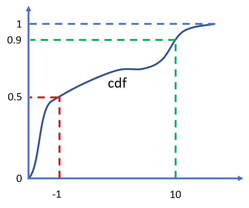
I have built a tool that creates a probability distribution (of a given family) from user-supplied quantiles, sometimes also called percentiles. Quantiles are points on the cumulative distribution function: (p,x) pairs such that P(X<x)=p. To illustrate what quantiles are, we can look at the example distribution below, which has a 50th percentile (or median) of -1 and a 90th percentile of 10.
A cumulative distribution function with a median of -1 and a 90th percentile of 10
Let’s run through some examples of how you can use this tool. At the end, I will discuss how it compares to other probability elicitation software, and why I think it’s a valuable addition.
Traditional distributions
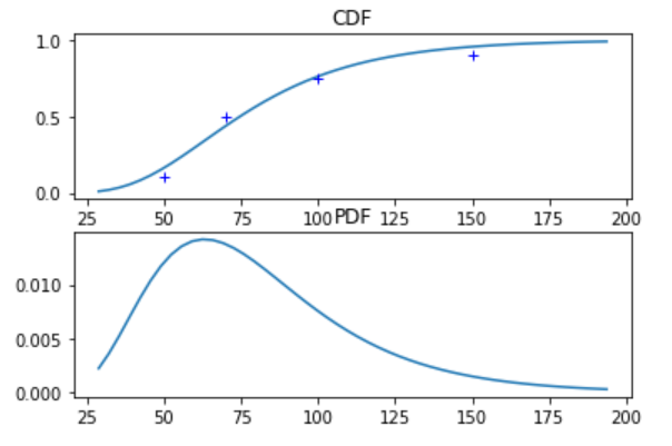
The tool supports the normal and lognormal distributions, and more of the usual distribution families could easily be added. The user supplies the distribution family, along with an arbitrary number of quantiles. If more quantiles are provided than the distribution has parameters (more than two in this case), the system is over-determined. The tool then uses least squares to find the best fit.
More than two quantiles provided, using least squares fit

Lognormal distribution
mu 4.313122980928514
sigma 0.409687416531683

quantiles:
0.01 28.79055927521217
0.1 44.17183774344628
0.25 56.64439363937313
0.5 74.67332855521319
0.75 98.44056294458953
0.9 126.2366766332274
0.99 193.67827989071688
Metalog distribution
The feature I am most excited about, however, is the support for a new type of distribution developed specifically for the purposes of flexible elicitation from quantiles, called the meta-logistic distribution. It was first described in Keelin 2016, which puts it at the cutting edge compared to the venerable normal distribution invented by Gauss and Laplace around 1810. The meta-logistic, or metalog for short, does not use traditional parameters. Instead, it can take on as many terms as the user provides quantiles, and adopts whatever shape is needed to fit these quantiles very closely. Closed-form expressions exist for its quantile function (the inverse of the CDF) and for its PDF. This leads to attractive computational properties (see footnote)1.
Keelin explains that
[t]he metalog distributions provide a convenient way to translate CDF data into smooth, continuous, closed-from distribution functions that can be used for real-time feedback to experts about the implications of their probability assessments.
The metalog quantile function is derived by modifying the logistic quantile function,
μ+sln1−yy for 0<y<1
by letting μ and s depend on y instead of being constant.
As Keelin writes, given a systematically increasing s as one moves from left to right, a right skewed distribution would result. And a systematically decreasing μ as one moves from left to right would make the distribution spikier in the middle with correspondingly heavier tails.
By modifying s and μ in ever more complex ways we can make the metalog take on almost any shape. In particular, in most cases the metalog CDF passes through all the provided quantiles exactly2. Moreover, we can specify the metalog to be unbounded, to have arbitrary bounds, or to be semi-bounded above or below.
Instead of thinking about which of several highly constraining distribution families to use, just choose the metalog and let your quantiles speak for themselves. As Keelin says:
one needs a distribution that has flexibility far beyond that of traditional distributions – one that enables “the data to speak for itself” in contrast to imposing unexamined and possibly inappropriate shape constraints on that data.
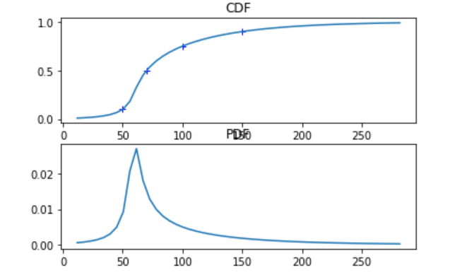
For example, we can fit an unbounded metalog to the same quantiles as above:
The metalog’s actual parameters (as opposed to the user-supplied quantiles) have no simple interpretation and are of no use unless the next piece of software you’re going to use knows what a metalog is. Therefore the program doesn’t return the parameters. Instead, if we want to manipulate this distribution, we can use the expressions of the PDF and CDF that the software provides, or alternatively export a large number of samples into another tool that accepts distributions described by a list of samples (such as the Monte Carlo simulation tool Guesstimate). By default, 5000 samples will be printed; you can copy and paste them.
Approaches to elicitation
How does this tool compare to other approaches for creating subjective belief distributions? Here are the strategies I’ve seen.
Belief intervals
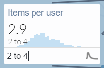
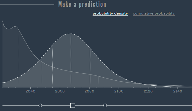
The first approach is to provide a belief interval that is mapped to some fixed quantiles, e.g. a 90% belief interval (between the 0.05 and 0.95 quantile) like on Guesstimate. Metaculus provides a graphical way to input the same data, allowing the user to drag the quantiles across a line under a graph of the PDF. This is the simplest and most user-friendly approach. The tool I built incorporates the belief interval approach while going beyond it in two ways. First, you can provide completely arbitrary quantiles, instead of specifically the 0.05 and 0.95 – or some other belief interval symmetric around 0.5. Second, you can provide more than two quantiles, which allows the user to query intuitive information about more parts of the distribution.
Guesstimate
Metaculus
Drawing
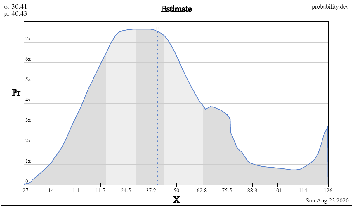
Another option is to draw the PDF on a canvas, in free form, using your mouse. This is the very innovative approach of probability.dev.3
probability.dev
Ought’s elicit
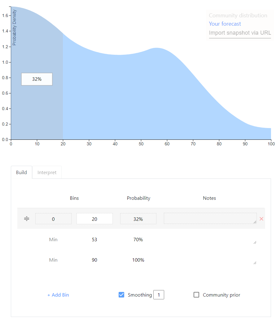
Ought’s elicit lets you provide quantiles like my tool, or equivalently bins with some probability mass in each bin4. The resulting distribution is by default piecewise uniform (the cdf is piecewise linear), but it’s possible to apply smoothing. It has all the features I want, the drawback is that it only supports bounded distributions5.
Elicit
Mixtures
A meta-level approach that can be applied to any of the above is to allow the user to specify a mixture distribution, a weighted average of distributions. For example, 1/3 weight on a normal(5,5) and 2/3 weight on a lognormal(1,0.75). My opinion on mixtures is that they are good if the user is thinking about the event disjunctively; for example, she may be envisioning two possible scenarios, each of which she has a distribution in mind for. But on Metaculus and Foretold my impression is that mixtures are often used to indirectly achieve a single distribution whose rough shape the user had in mind originally.
The future
This is an exciting space with many recent developments. Guesstimate, Metaculus, Elicit and the metalog distribution have all been created in the last 5 years.
For the quantile function expression, see Keelin 2016, definition 1. The fact that this is in closed form means, first, that sampling randomly from the distribution is computationally trivial. We can use the inverse transform method: we take random samples from a uniform distribution over [0,1] and plug them into the quantile function. Second, plotting the CDF for a certain range of probabilities (e.g. from 1% to 99%) is also easy.
The expression for the PDF is unusual in that it is a function of the cumulative probability p∈(0,1), instead of a function of values of the random variable. See Keelin 2016, definition 2. As Keelin explains (p. 254), to plot the PDF as is customary we can use the quantile function q(p) on the horizontal axis and the PDF expression f(p) on the vertical axis, and vary p in, for example, [0.01,0.99] to produce the corresponding values on both axes.
Hence, for (i) querying the quantile function of the fitted metalog, sampling, and plotting the CDF, and (ii) plotting the PDF, everything can be done in closed form.
To query the CDF, however, numerical equation solving is applied. Since the quantile function is differentiable, Newton’s method can be applied and is fast. (Numerical equation solving is also used to query the PDF as a function of values of the random variable – but I don’t see why one would need densities except for plotting.) ↩
In most cases, there exists a metalog whose CDF passes through all the provided quantiles exactly. In that case, there exists an expression of the metalog parameters that is in closed form as a function of the quantiles (“a=Y−1x”, Keelin 2016, p. 253. Keelin denotes the metalog parameters a, the matrix Y is a simple function of the quantiles’ y-coordinates, and the vector x contains the quantiles’ x-coordinates. The metalog parameters a are the numbers that are used to modify the logistic quantile function. This modification is done according to equation 6 on p. 254.)
If there is no metalog that fits the quantiles exactly (i.e. the expression for a above does not imply a valid probability distribution), we have to use optimization to find the feasible metalog that fits the quantiles most closely. In this software implementation, “most closely” is defined as minimizing the absolute differences between the quantiles and the CDF (see here for more discussion).
In my experience, if a small number of quantiles describing a PDF with sharp peaks are provided, the closest feasible metalog fit to the quantiles may not pass through all the quantiles exactly. ↩
Drawing the PDF instead of the CDF makes it difficult to hit quantiles. But drawing the CDF would probably be less intuitive – I often have the rough shape of the PDF in mind, but I never have intuitions about the rough shape of the CDF. The canvas-based approach also runs into difficulty with the tail of unbounded distributions. Overall I think it’s very cool but I haven’t found it that practical. ↩
To provide quantiles, simply leave the Min field empty – it defaults to the left bound of the distribution. ↩
I suspect this is a fundamental problem of the approach of starting with piecewise uniforms and adding smoothing. You need the tails of the CDF to asymptote towards 0 and 1, but it’s hard to find a mathematical function that does this while also (i) having the right probability mass under the tail (ii) stitching onto the piecewise uniforms in a natural way. I’d love to be proven wrong, though; the user interface and user experience on Elicit are really nice. (I’m aware that Elicit allows for ‘open-ended’ distributions, where probability mass can be assigned to an out-of-bounds outcome, but one cannot specify how that mass is distributed inside the out-of-bounds interval(s). So there is no true support for unbounded distributions. The ‘out-of-bounds’ feature exists because Elicit seems to be mainly intended as an add-on to Metaculus, which supports such ‘open-ended’ distributions but no truly unbounded ones.) ↩
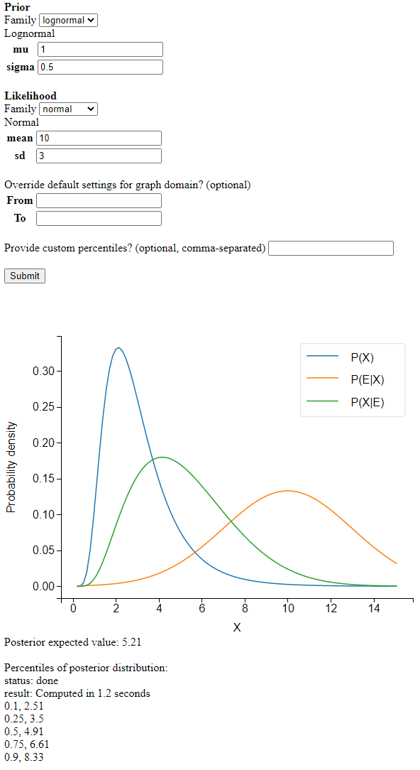
I wrote a Python app to apply Bayes’ rule to continuous distributions. It looks like this:
Screenshot
I’m learning a lot about numerical analysis from this project. The basic idea is simple:
defunnormalized_posterior_pdf(x):returnprior.pdf(x)*likelihood.pdf(x)# integrate unnormalized_posterior_pdf over the reals
normalization_constant=integrate.quad(unnormalized_posterior_pdf,-np.inf,np.inf)[0]defposterior_pdf(x):returnunnormalized_posterior_pdf(x)/normalization_constant
However, when testing my code on complicated distributions, I ran into some interesting puzzles.
A first set of problems was caused by the SciPy numerical integration routines that my program relies on. They were sometimes returning incorrect results or RuntimeErorrs. These problems appeared when the integration routines had to deal with ‘extreme’ values: small normalization constants or large inputs into the cdf function. I eventually learned to hold the integration algorithm’s hand a little bit and show it where to go.
A second set of challenges had to do with how long my program took to run: sometimes 30 seconds to return the percentiles of the posterior distribution. While 30 seconds might be acceptable for someone who desperately needed that bayesian update, I didn’t want my tool to feel like a punch card mainframe. I eventually managed to make the program more than 10 times faster. The tricks I used all followed the same strategy. In order to make it less expensive to repeatedly evaluate the posterior’s cdf by numerical integration, I tried to find ways to make the interval to integrate narrower.
You can follow along with all the tests described in this post using this file, whereas the code doing the calculations for the webapp is here.
Small normalization constants
When the prior and likelihood are far apart, the unnormalized posterior takes tiny values.
It turns out that SciPy’s integration routine, integrate.quad, (incidentally, written in actual Fortran!) has trouble integrating such a low-valued pdf.
prior=stats.lognorm(s=.5,scale=math.exp(.5))# a lognormal(.5,.5) in SciPy notation
likelihood=stats.norm(20,1)classPosterior_scipyrv(stats.rv_continuous):def__init__(self,d1,d2):super(Posterior_scipyrv,self).__init__()self.d1=d1self.d2=d2self.normalization_constant=integrate.quad(self.unnormalized_pdf,-np.inf,np.inf)[0]defunnormalized_pdf(self,x):returnself.d1.pdf(x)*self.d2.pdf(x)def_pdf(self,x):returnself.unnormalized_pdf(x)/self.normalization_constantposterior=Posterior_scipyrv(prior,likelihood)print('normalization constant:',posterior.normalization_constant)print("CDF values:")foriinrange(30):print(i,posterior.cdf(i))
The cdf converges to… 52,477. This is not so good.
Because the cdf does converge, but to an incorrect value, we can conclude that the normalization constant is to blame. Because the cdf converges to a number greater than 1, posterior.normalization_constant, about 3e-12, is an underestimate of the true value.
If we shift the likelihood distribution just a little bit to the left, to likelihood = stats.norm(18,1), the cdf converges correctly, and we get a normalization constant of about 6e-07. Obviously, the normalization constant should not jump five orders of magnitude from 6e-07 to 3e-12 as a result of this small shift.
The program is not integrating the unnormalized pdf correctly.
Difficulties with integration usually have to do with the shape of the function. If your integrand zig-zags up and down a lot, the algorithm may miss some of the peaks. But here, the shape of the posterior is almost the same whether we use stats.norm(18,1) or stats.norm(20,1)1. So the problem really seems to occur once we are far enough in the tails of the prior that the unnormalized posterior pdf takes values below a certain absolute (rather than relative) threshold. I don’t yet understand why. Perhaps some of the values are becoming too small to be represented with standard floating point numbers.
This seems rather bizarre, but here’s a piece of evidence that really demonstrates that low absolute values are what’s tripping up the integration routine that calculates the normalization constant. We just multiply the unnormalized pdf by 10000 (which will cancel out once we normalize).
We take a prior and likelihood that are unproblematically close together:
prior=stats.lognorm(s=.5,scale=math.exp(.5))# a lognormal(.5,.5) in SciPy notation
likelihood=stats.norm(5,1)posterior=Posterior_scipyrv(prior,likelihood)foriinrange(100):print(i,posterior.cdf(i))
At first, the cdf goes to 1 as expected, but suddenly all hell breaks loose and the cdf decreases to some very tiny values:
What’s going on? When asked to integrate the pdf from minus infinity up to some large value like 25, quad doesn’t know where to look for the probability mass. When the upper bound of the integral is in an area with still enough probability mass, like 23 or 24 in this example, quad finds its way to the mass. But if you ask it to find a peak very far away, it fails.
A piece of confirmatory evidence is that if we make the peak spikier and harder to find, by setting the likelihood’s standard deviation to 0.5 instead of 1, the cdf fails earlier:
22 1.000000000000232
23 2.9116983489798973e-12
We need to hold the integration algorithm’s hand and show it where on the real line the peak of the distribution is located. In SciPy’s quad, you can supply the points argument to point out places ‘where local difficulties of the integrand may occur’, but only when the integration interval is finite. The solution I came up with is to split the interval into two halves.
defsplit_integral(f,splitpoint,integrate_to):a,b=-np.inf,np.infifintegrate_to<splitpoint:# just return the integral normally
returnintegrate.quad(f,a,integrate_to)[0]else:integral_left=integrate.quad(f,a,splitpoint)[0]integral_right=integrate.quad(f,splitpoint,integrate_to)[0]returnintegral_left+integral_right
This definitely won’t work for every difficult integral, but should help for many cases where most of the probability mass is not too far from the splitpoint.
For splitpoint, a simple choice is the average of the prior and likelihood’s expected values.
So far I’ve only talked about problems that cause the program to return the wrong answer. This section is about a problem that only causes inefficiency, at least when it isn’t combined with other problems.
If you don’t specify the support of a continuous random variable in SciPy, it defaults to the entire real line. This leads to inefficiency when querying quantiles of the distribution. If I want to know the 50th percentile of my distribution, I call ppf(0.5). As I described previously, ppf works by numerically solving the equation cdf(x)=0.5. The ppf method automatically passes the support of the distribution into the equation solver and tells it to only look for solutions inside the support. When a distribution’s support is a subset of the reals, searching over the entire reals is inefficient.
To remedy this, we can define the support of the posterior as the intersection of the prior and likelihood’s support. For this we need a small function that calculates the intersection of two intervals.
defintersect_intervals(two_tuples):d1,d2=two_tuplesd1_left,d1_right=d1[0],d1[1]d2_left,d2_right=d2[0],d2[1]ifd1_right<d2_leftord2_right<d2_left:raiseValueError("the distributions have no overlap")intersect_left,intersect_right=max(d1_left,d2_left),min(d1_right,d2_right)returnintersect_left,intersect_right
We can then call this function:
classPosterior_scipyrv(stats.rv_continuous):def__init__(self,d1,d2):super(Posterior_scipyrv,self).__init__()a1,b1=d1.support()a2,b2=d2.support()# 'a' and 'b' are scipy's names for the bounds of the support
self.a,self.b=intersect_intervals([(a1,b1),(a2,b2)])
To test this, let’s use a beta distribution, which is defined on [0,1]:
We know that the posterior will also be defined on [0,1]. By defining the support of the posterior inside the the __init__ method of Posterior_scipyrv, we give SciPy access to this information.
We can time the resulting speedup in calculating posterior.ppf(0.99):
print("support:",posterior.support())s=time.time()print("result:",posterior.ppf(0.99))e=time.time()print(e-s,'seconds to evalute ppf')
support: (-inf, inf)
result: 0.9901821216897447
3.8804399967193604 seconds to evalute ppf

support: (0.0, 1.0)
result: 0.9901821216904315
0.40013647079467773 seconds to evalute ppf
We’re able to achieve an almost 10x speedup, with very meaningful impact on user experience. For less extreme quantiles, like posterior.ppf(0.5), I still get a 2x speedup.
The lack of properly defined support causes only inefficiency if we continue to use split_integral to calculate the cdf. But if we leave the cdf problem unaddressed, it can combine with the too-wide support to produce outright errors.
For example, suppose we use a beta distribution again for the prior, but we don’t use the split integral for the cdf, and nor do we define the support of the posterior as [0,1] instead of IR.
When the integration algorithm is looking over all of (−∞,3.4], it has no way of knowing that all the probability mass is in [0,1]. The posterior distribution has only one big bump in the middle, so it’s not surprising that the algorithm misses it.
If we now ask the equation solver in ppf to find quantiles, without telling it that all the solutions are in [0,1], it will try to evaluate points like cdf(4), which return 0 – but ppf is assuming that the cdf is increasing. This leads to catastrophe. Running posterior.ppf(0.5) gives a RuntimeError: Failed to converge after 100 iterations. At first I wondered why beta distributions would always give me RuntimeErrors…
Optimization: CDF memoization
When we call ppf, the equation solver calls cdf for the same distribution many times. This suggests we could optimize things further by storing known cdf values, and only doing the integration from the closest known value to the desired value. This will result in the same number of integration calls, but each will be over a smaller interval (except the first). This is a form of memoization.
We can also squeeze out some additional speedup by considering the cdf to be 1 forevermore once it reaches values close to 1.
classPosterior_scipyrv(stats.rv_continuous):def_cdf(self,x):# exploit considering the cdf to be 1
# forevermore once it reaches values close to 1
forx_lookupinself.cdf_lookup:ifx_lookup<xandnp.around(self.cdf_lookup[x_lookup],5)==1.0:return1# check lookup table for largest integral already computed below x
sortedkeys=sorted(self.cdf_lookup,reverse=True)forkeyinsortedkeys:#find the greatest key less than x
ifkey<x:ret=self.cdf_lookup[key]+integrate.quad(self.pdf,key,x)[0]self.cdf_lookup[float(x)]=retreturnret# Initial run
ret=split_integral(self.pdf,self.splitpoint,x)self.cdf_lookup[float(x)]=retreturnret
If we return to our earlier prior and likelihood
prior=stats.lognorm(s=.5,scale=math.exp(.5))# a lognormal(.5,.5) in SciPy notation
likelihood=stats.norm(5,1)
and make calls to ppf([0.1, 0.9, 0.25, 0.75, 0.5]), the memoization gives us about a 5x speedup:
memoization False
[2.63571613 5.18538207 3.21825988 4.56703016 3.88645864]
length of lookup table: 0
2.1609253883361816 seconds to evalute ppf

memoization True
[2.63571613 5.18538207 3.21825988 4.56703016 3.88645864]
length of lookup table: 50
0.4501194953918457 seconds to evalute ppf
These speed gains again occur over a range that makes quite a difference to user experience: going from multiple seconds to a fraction of a second.
Optimization: ppf with bounds
In my webapp, I give the user some standard percentiles: 0.1, 0.25, 0.5, 0.75, 0.9.
Given that ppf works by numerical equation solving on the cdf, if we give the solver a smaller domain in which to look for the solutions, it should find them more quickly. When we calculate multiple percentiles, each percentile we calculate helps us close in on the others. If the 0.1 percentile is 12, we have a lower bound of 12 for on any percentile p>0.1. If we have already calculated a percentile on each side, we have both a lower and upper bound.
We can’t directly pass the bounds to ppf, so we have to wrap the method, which is found here in the source code. (To help us focus, I give a simplified presentation below that cuts out some code designed to deal with unbounded supports. The code below will not run correctly).
classPosterior_scipyrv(stats.rv_continuous):defppf_with_bounds(self,q,leftbound,rightbound):left,right=self._get_support()# SciPy ppf code to deal with case where left or right are infinite.
# Omitted for simplicity.
ifleftboundisnotNone:left=leftboundifrightboundisnotNone:right=rightbound# brentq is the equation solver (from Brent 1973)
# _ppf_to_solve is simply cdf(x)-q, since brentq
# finds points where a function equals 0
returnoptimize.brentq(self._ppf_to_solve,left,right,args=q)
To get some bounds, we run the extreme percentiles first, narrowing in on the middle percentiles from both sides. For example in 0.1, 0.25, 0.5, 0.75, 0.9, we want to evaluate them in this order: 0.1, 0.9, 0.25, 0.75, 0.5. We store each of the answers in result.
classPosterior_scipyrv(stats.rv_continuous):defcompute_percentiles(self,percentiles_list):result={}percentiles_list.sort()# put percentiles in the order they should be computed
percentiles_reordered=sum(zip(percentiles_list,reversed(percentiles_list)),())[:len(percentiles_list)]# see https://stackoverflow.com/a/17436999/8010877
defget_bounds(dict,p):# get bounds (if any) from already computed `result`s
keys=list(dict.keys())keys.append(p)keys.sort()i=keys.index(p)ifi!=0:leftbound=dict[keys[i-1]]else:leftbound=Noneifi!=len(keys)-1:rightbound=dict[keys[i+1]]else:rightbound=Nonereturnleftbound,rightboundforpinpercentiles_reordered:leftbound,rightbound=get_bounds(result,p)res=self.ppf_with_bounds(p,leftbound,rightbound)result[p]=np.around(res,2)sorted_result={key:valueforkey,valueinsorted(result.items())}returnsorted_result
The speedup is relatively minor when calculating just 5 percentiles.
Using ppf bounds? True
total time to compute percentiles: 3.1997928619384766 seconds

Using ppf bounds? False
total time to compute percentiles: 3.306936264038086 seconds
It grows a little bit with the number of percentiles, but calculating a large number of percentiles would just lead to information overload for the user.
This was surprising to me. Using the bounds dramatically cuts the width of the interval for equation solving, but leads to only a minor speedup. Using fulloutput=True in optimize.brentq, we can see the number of function evaluations that brentq uses. This lets us see that the number of evaluations needed by brentq is highly non-linear in the width of the interval. The solver gets quite close to the solution very quickly, so giving it a narrow interval hardly helps.
Using ppf bounds? True
brentq looked between 0.0 10.0 and took 11 iterations
brentq looked between 0.52 10.0 and took 13 iterations
brentq looked between 0.52 2.24 and took 8 iterations
brentq looked between 0.81 2.24 and took 9 iterations
brentq looked between 0.81 1.73 and took 7 iterations
total time to compute percentiles: 3.1997928619384766 seconds

Using ppf bounds? False
brentq looked between 0.0 10.0 and took 11 iterations
brentq looked between 0.0 10.0 and took 10 iterations
brentq looked between 0.0 10.0 and took 10 iterations
brentq looked between 0.0 10.0 and took 10 iterations
brentq looked between 0.0 10.0 and took 9 iterations
total time to compute percentiles: 3.306936264038086 seconds
Brent’s method is a very efficient equation solver.
It has a very similar shape to the likelihood (because the likelihood has much lower variance than the prior). ↩